Estimation of Price Surfaces¶

This notebook outlines how to use the lowess.SmoothDates model to fit a LOWESS estimate where the coefficients change over time.

Imports¶

import pandas as pd
import numpy as np

import matplotlib.pyplot as plt
import seaborn as sns

import pickle

from moepy import lowess, moe, eda, surface

Data Preparation¶

We'll first load the data in

df_EI = pd.read_csv('../data/ug/electric_insights.csv')

df_EI['local_datetime'] = pd.to_datetime(df_EI['local_datetime'], utc=True)
df_EI = df_EI.set_index('local_datetime')

df_EI.head()

local_datetime	day_ahead_price	SP	imbalance_price	valueSum	temperature	TCO2_per_h	gCO2_per_kWh	nuclear	coal	...	demand	pumped_storage	wind_onshore	wind_offshore	french	irish
2010-01-01 00:00:00+00:00	32.91	1	55.77	55.77	1.1	16268	429	7.897	9.902	...	37.948	-0.435	nan	nan	1.963	-0.234
2010-01-01 00:30:00+00:00	33.25	2	59.89	59.89	1.1	16432	430	7.897	10.074	...	38.227	-0.348	nan	nan	1.974	-0.236
2010-01-01 01:00:00+00:00	32.07	3	53.15	53.15	1.1	16318	431	7.893	10.049	...	37.898	-0.424	nan	nan	1.983	-0.236
2010-01-01 01:30:00+00:00	31.99	4	38.48	38.48	1.1	15768	427	7.896	9.673	...	36.918	-0.575	nan	nan	1.983	-0.236
2010-01-01 02:00:00+00:00	31.47	5	37.7	37.7	1.1	15250	424	7.9	9.37	...	35.961	-0.643	nan	nan	1.983	-0.236

Then extract the relevant time-series for our analysis

df_EI_model = df_EI[['day_ahead_price', 'demand', 'solar', 'wind']].dropna()

s_price = df_EI_model['day_ahead_price']
s_dispatchable = df_EI_model['demand'] - df_EI_model[['solar', 'wind']].sum(axis=1)

s_dispatchable.head()

local_datetime
2010-01-01 00:00:00+00:00    36.902
2010-01-01 00:30:00+00:00    37.177
2010-01-01 01:00:00+00:00    36.834
2010-01-01 01:30:00+00:00    35.810
2010-01-01 02:00:00+00:00    34.850
dtype: float64

Model Fitting¶

Before we fit our model we need to create an array of dates which will act as the anchor locations of our time-adapative model, at each of these a separate LOWESS curve will be fitted.

reg_dates_start = '2010-01-01'
reg_dates_end = '2021-01-01'
reg_dates_freq = '13W'

reg_dates = pd.date_range(reg_dates_start,  reg_dates_end, freq=reg_dates_freq)

reg_dates[:5]

DatetimeIndex(['2010-01-03', '2010-04-04', '2010-07-04', '2010-10-03',
               '2011-01-02'],
              dtype='datetime64[ns]', freq='13W-SUN')

We're now ready to fit our model!

As well as passing in the anchor dates we provide the dt_idx, x, and y arrays from our data. We'll also pass an optional parameter that specifies the number of LOWESS anchor points in the x dimension (reducing the computation required).

smooth_dates = lowess.SmoothDates()

smooth_dates.fit(
    dt_idx=s_dispatchable.index, 
    x=s_dispatchable.values, 
    y=s_price.values, 
    reg_dates=reg_dates, 
    num_fits=15
)

100%|â–ˆâ–ˆâ–ˆâ–ˆâ–ˆâ–ˆâ–ˆâ–ˆâ–ˆâ–ˆâ–ˆâ–ˆâ–ˆâ–ˆâ–ˆâ–ˆâ–ˆâ–ˆâ–ˆâ–ˆâ–ˆâ–ˆâ–ˆâ–ˆâ–ˆâ–ˆâ–ˆâ–ˆâ–ˆâ–ˆâ–ˆâ–ˆâ–ˆâ–ˆâ–ˆâ–ˆâ–ˆâ–ˆâ–ˆâ–ˆâ–ˆâ–ˆâ–ˆâ–ˆâ–ˆâ–ˆâ–ˆâ–ˆâ–ˆâ–ˆâ–ˆâ–ˆâ–ˆâ–ˆâ–ˆâ–ˆâ–ˆâ–ˆâ–ˆâ–ˆâ–ˆâ–ˆâ–ˆâ–ˆâ–ˆâ–ˆâ–ˆâ–ˆâ–ˆâ–ˆâ–ˆâ–ˆâ–ˆâ–ˆâ–ˆâ–ˆâ–ˆâ–ˆâ–ˆâ–ˆâ–ˆâ–ˆ| 45/45 [02:52<00:00,  3.83s/it]

As with any sklearn style model once we've used fit we're ready to predict, unlike standard sklearn models however we're returned the prediction of the model surface (as a matrix) rather than a single array.

x_pred = np.linspace(8, 60, 521)
dt_pred = pd.date_range('2010-01-01', '2021-01-01')

df_pred = smooth_dates.predict(x_pred=x_pred, dt_pred=dt_pred)

df_pred.head()

Unnamed: 0	2010-01-01	2010-01-02	2010-01-03	2010-01-04	2010-01-05	2010-01-06	2010-01-07	2010-01-08	2010-01-09	2010-01-10	...	2020-12-23	2020-12-24	2020-12-25	2020-12-26	2020-12-27	2020-12-28	2020-12-29	2020-12-30	2020-12-31	2021-01-01
8	18.9567	18.9668	18.9769	18.9869	18.9969	19.0069	19.0169	19.0269	19.0368	19.0468	...	5.42077	5.41609	5.41138	5.40666	5.40192	5.39717	5.3924	5.38762	5.38283	5.37802
8.1	19.0524	19.0624	19.0725	19.0825	19.0925	19.1025	19.1124	19.1224	19.1323	19.1422	...	5.66763	5.66297	5.65829	5.6536	5.64889	5.64416	5.63942	5.63467	5.6299	5.62511
8.2	19.1479	19.158	19.168	19.178	19.188	19.198	19.2079	19.2178	19.2278	19.2377	...	5.91447	5.90984	5.90518	5.90051	5.89583	5.89113	5.88642	5.88169	5.87695	5.87219
8.3	19.2436	19.2536	19.2636	19.2736	19.2835	19.2935	19.3034	19.3133	19.3232	19.3331	...	6.16155	6.15694	6.15231	6.14767	6.14301	6.13834	6.13365	6.12895	6.12424	6.11951
8.4	19.3392	19.3492	19.3592	19.3691	19.3791	19.389	19.3989	19.4088	19.4187	19.4286	...	6.40911	6.40453	6.39993	6.39531	6.39068	6.38604	6.38138	6.3767	6.37201	6.36731

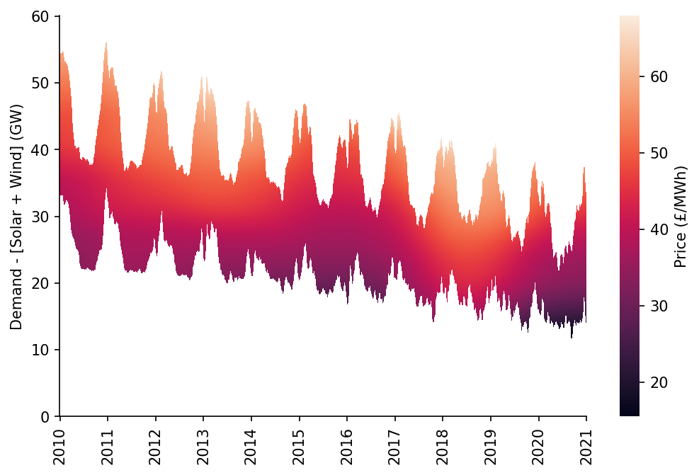
We'll quickly visualise this surface, masking areas where no data was available

# Preparing mask
df_dispatchable_lims = moe.construct_dispatchable_lims_df(s_dispatchable)
df_pred_mask = moe.construct_pred_mask_df(df_pred, df_dispatchable_lims)

# Plotting
fig, ax = plt.subplots(dpi=150, figsize=(8, 5))

htmp = sns.heatmap(df_pred[10:60].where(df_pred_mask[10:60], np.nan).iloc[::-1], ax=ax, cbar_kws={'label': 'Price (Â£/MWh)'})

moe.set_ticks(ax, np.arange(0, 70, 10), axis='y')
moe.set_date_ticks(ax, '2010-01-01', '2021-01-01', freq='1YS', date_format='%Y', axis='x')

for _, spine in htmp.spines.items():
    spine.set_visible(True)
eda.hide_spines(ax)

ax.set_ylabel('Demand - [Solar + Wind] (GW)')

C:\Users\Ayrto\AppData\Roaming\Python\Python39\site-packages\sklearn\utils\validation.py:63: FutureWarning: Arrays of bytes/strings is being converted to decimal numbers if dtype='numeric'. This behavior is deprecated in 0.24 and will be removed in 1.1 (renaming of 0.26). Please convert your data to numeric values explicitly instead.
  return f(*args, **kwargs)





Text(107.08333333333331, 0.5, 'Demand - [Solar + Wind] (GW)')

png

The model is also pkl compatible, allowing it to be easily saved for later use

model_fp = '../data/ug/GB_example_model.pkl'

pickle.dump(smooth_dates, open(model_fp, 'wb'))

A separate function - surface.fit_models - provides a highly flexible interface for orchestrating several model fits. The fitted models are saved using the name specified as the key in the model_definitions dictionary.

model_definitions = {
    'GB_detailed_example_model': {
        'dt_idx': s_dispatchable.index,
        'x': s_dispatchable.values,
        'y': s_price.values,
        'reg_dates_start': '2020-01-01',
        'reg_dates_end': '2021-01-01',
        'reg_dates_freq': '26W', 
        'frac': 0.3, 
        'num_fits': 10,
        'dates_smoothing_value': 26, 
        'dates_smoothing_units': 'W',
        'fit_kwarg_sets': surface.get_fit_kwarg_sets(qs=[0.5])
    }
}

surface.fit_models(model_definitions, '../data/ug')

GB_detailed_example_model:   0%|                                                                 | 0/2 [00:00<?, ?it/s]
  0%|                                                                                            | 0/2 [00:00<?, ?it/s][A
 50%|â–ˆâ–ˆâ–ˆâ–ˆâ–ˆâ–ˆâ–ˆâ–ˆâ–ˆâ–ˆâ–ˆâ–ˆâ–ˆâ–ˆâ–ˆâ–ˆâ–ˆâ–ˆâ–ˆâ–ˆâ–ˆâ–ˆâ–ˆâ–ˆâ–ˆâ–ˆâ–ˆâ–ˆâ–ˆâ–ˆâ–ˆâ–ˆâ–ˆâ–ˆâ–ˆâ–ˆâ–ˆâ–ˆâ–ˆâ–ˆâ–ˆâ–ˆ                                          | 1/2 [00:48<00:48, 48.47s/it][A
100%|â–ˆâ–ˆâ–ˆâ–ˆâ–ˆâ–ˆâ–ˆâ–ˆâ–ˆâ–ˆâ–ˆâ–ˆâ–ˆâ–ˆâ–ˆâ–ˆâ–ˆâ–ˆâ–ˆâ–ˆâ–ˆâ–ˆâ–ˆâ–ˆâ–ˆâ–ˆâ–ˆâ–ˆâ–ˆâ–ˆâ–ˆâ–ˆâ–ˆâ–ˆâ–ˆâ–ˆâ–ˆâ–ˆâ–ˆâ–ˆâ–ˆâ–ˆâ–ˆâ–ˆâ–ˆâ–ˆâ–ˆâ–ˆâ–ˆâ–ˆâ–ˆâ–ˆâ–ˆâ–ˆâ–ˆâ–ˆâ–ˆâ–ˆâ–ˆâ–ˆâ–ˆâ–ˆâ–ˆâ–ˆâ–ˆâ–ˆâ–ˆâ–ˆâ–ˆâ–ˆâ–ˆâ–ˆâ–ˆâ–ˆâ–ˆâ–ˆâ–ˆâ–ˆâ–ˆâ–ˆâ–ˆâ–ˆâ–ˆâ–ˆ| 2/2 [01:40<00:00, 50.10s/it][A
GB_detailed_example_model:  50%|â–ˆâ–ˆâ–ˆâ–ˆâ–ˆâ–ˆâ–ˆâ–ˆâ–ˆâ–ˆâ–ˆâ–ˆâ–ˆâ–ˆâ–ˆâ–ˆâ–ˆâ–ˆâ–ˆâ–ˆâ–ˆâ–ˆâ–ˆâ–ˆâ–ˆâ–ˆâ–ˆâ–ˆ                            | 1/2 [01:40<01:40, 100.48s/it]
  0%|                                                                                            | 0/2 [00:00<?, ?it/s][A
 50%|â–ˆâ–ˆâ–ˆâ–ˆâ–ˆâ–ˆâ–ˆâ–ˆâ–ˆâ–ˆâ–ˆâ–ˆâ–ˆâ–ˆâ–ˆâ–ˆâ–ˆâ–ˆâ–ˆâ–ˆâ–ˆâ–ˆâ–ˆâ–ˆâ–ˆâ–ˆâ–ˆâ–ˆâ–ˆâ–ˆâ–ˆâ–ˆâ–ˆâ–ˆâ–ˆâ–ˆâ–ˆâ–ˆâ–ˆâ–ˆâ–ˆâ–ˆ                                          | 1/2 [00:02<00:02,  2.60s/it][A
100%|â–ˆâ–ˆâ–ˆâ–ˆâ–ˆâ–ˆâ–ˆâ–ˆâ–ˆâ–ˆâ–ˆâ–ˆâ–ˆâ–ˆâ–ˆâ–ˆâ–ˆâ–ˆâ–ˆâ–ˆâ–ˆâ–ˆâ–ˆâ–ˆâ–ˆâ–ˆâ–ˆâ–ˆâ–ˆâ–ˆâ–ˆâ–ˆâ–ˆâ–ˆâ–ˆâ–ˆâ–ˆâ–ˆâ–ˆâ–ˆâ–ˆâ–ˆâ–ˆâ–ˆâ–ˆâ–ˆâ–ˆâ–ˆâ–ˆâ–ˆâ–ˆâ–ˆâ–ˆâ–ˆâ–ˆâ–ˆâ–ˆâ–ˆâ–ˆâ–ˆâ–ˆâ–ˆâ–ˆâ–ˆâ–ˆâ–ˆâ–ˆâ–ˆâ–ˆâ–ˆâ–ˆâ–ˆâ–ˆâ–ˆâ–ˆâ–ˆâ–ˆâ–ˆâ–ˆâ–ˆâ–ˆâ–ˆâ–ˆâ–ˆ| 2/2 [00:05<00:00,  2.59s/it][A
GB_detailed_example_model: 100%|â–ˆâ–ˆâ–ˆâ–ˆâ–ˆâ–ˆâ–ˆâ–ˆâ–ˆâ–ˆâ–ˆâ–ˆâ–ˆâ–ˆâ–ˆâ–ˆâ–ˆâ–ˆâ–ˆâ–ˆâ–ˆâ–ˆâ–ˆâ–ˆâ–ˆâ–ˆâ–ˆâ–ˆâ–ˆâ–ˆâ–ˆâ–ˆâ–ˆâ–ˆâ–ˆâ–ˆâ–ˆâ–ˆâ–ˆâ–ˆâ–ˆâ–ˆâ–ˆâ–ˆâ–ˆâ–ˆâ–ˆâ–ˆâ–ˆâ–ˆâ–ˆâ–ˆâ–ˆâ–ˆâ–ˆâ–ˆâ–ˆ| 2/2 [01:45<00:00, 52.91s/it]