Marginal Price Curve Estimation for Dispatchable Power in Great Britain
![]()
In this example we'll estimate the marginal price curve over the last two months for dispatchable power in Great Britain using data from Electric Insights.
Imports
import numpy as np
import pandas as pd

import matplotlib.pyplot as plt

from moepy import retrieval, eda, lowess
Data Loading
We'll start by loading in the necessary data from Electric Insights
%%time

current_dt = pd.Timestamp.now()
start_date = (current_dt-pd.Timedelta(weeks=8)).strftime('%Y-%m-%d %H:%M')
end_date = current_dt.strftime('%Y-%m-%d %H:%M')

renaming_dict = {
    'pumpedStorage' : 'pumped_storage',
    'northernIreland' : 'northern_ireland',
    'windOnshore': 'wind_onshore',
    'windOffshore': 'wind_offshore',
    'prices_ahead' : 'day_ahead_price',
    'prices' : 'imbalance_price',
    'temperatures' : 'temperature',
    'totalInGperkWh' : 'gCO2_per_kWh',
    'totalInTperh' : 'TCO2_per_h'
}

df = retrieval.retrieve_streams_df(start_date, end_date, renaming_dict=renaming_dict)

df.head()
Wall time: 7.75 s
| local_datetime | day_ahead_price | SP | imbalance_price | valueSum | temperature | TCO2_per_h | gCO2_per_kWh | nuclear | biomass | coal | ... | demand | pumped_storage | wind_onshore | wind_offshore | belgian | dutch | french | ireland | northern_ireland | irish |
|---|---|---|---|---|---|---|---|---|---|---|---|---|---|---|---|---|---|---|---|---|---|
| 2021-02-01 00:00:00+00:00 | 51.99 | 1 | 68.95 | 68.95 | 2.9 | 4797.76 | 175.8 | 5.564 | 1.945 | 0.465 | ... | 27.291 | 0 | 3.02828 | 3.51436 | 0.902 | 0 | 1.806 | 0 | 0.018 | -0.05 |
| 2021-02-01 00:30:00+00:00 | 54.19 | 2 | 69 | 69 | 2.9 | 5149.7 | 186.031 | 5.559 | 1.963 | 0.563 | ... | 27.682 | 0 | 2.90388 | 3.44746 | 0.902 | 0 | 1.806 | 0 | 0.016 | 0.016 |
| 2021-02-01 01:00:00+00:00 | 55.07 | 3 | 75 | 75 | 2.9 | 5177.97 | 189.309 | 5.565 | 2.077 | 0.68 | ... | 27.352 | 0 | 2.76413 | 3.36153 | 0.952 | 0 | 1.906 | 0 | 0.018 | 0.018 |
| 2021-02-01 01:30:00+00:00 | 56.3 | 4 | 72 | 72 | 2.9 | 5131.08 | 190.892 | 5.563 | 2.122 | 0.716 | ... | 26.8796 | 0 | 2.62404 | 3.19386 | 0.952 | 0 | 1.906 | 0 | 0.016 | 0.016 |
| 2021-02-01 02:00:00+00:00 | 56.71 | 5 | 75 | 75 | 2.9 | 5105.37 | 193.368 | 5.561 | 2.134 | 0.718 | ... | 26.4023 | 0 | 2.41751 | 2.93459 | 0.926 | 0 | 1.906 | 0 | 0.018 | 0.018 |
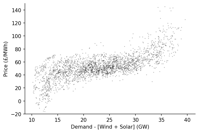
We'll quickly visualise the relationship between price and dispatchable load for each half-hour period
df_model = df[['day_ahead_price', 'demand', 'solar', 'wind']].dropna().astype(float)

s_price = df_model['day_ahead_price']
s_dispatchable = df_model['demand'] - df_model[['solar', 'wind']].sum(axis=1)

# Plotting
fig, ax = plt.subplots(dpi=150)

ax.scatter(s_dispatchable, s_price, s=0.5, alpha=0.25, color='k')

ax.set_ylim(-20, 150)
eda.hide_spines(ax)
ax.set_xlabel('Demand - [Wind + Solar] (GW)')
ax.set_ylabel('Price (£/MWh)')
Text(0, 0.5, 'Price (£/MWh)')
Marginal Price Curve Estimation
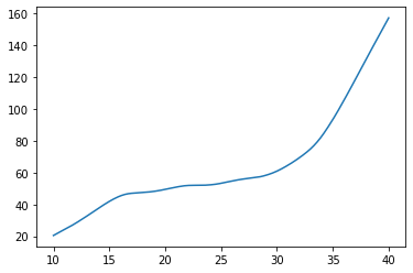
We're now ready to fit our LOWESS model
x_pred = np.linspace(10, 40, 301)

y_pred = lowess.lowess_fit_and_predict(s_dispatchable.values,
                                       s_price.values,
                                       frac=0.25,
                                       num_fits=25,
                                       x_pred=x_pred)

pd.Series(y_pred, index=x_pred).plot()
<AxesSubplot:>
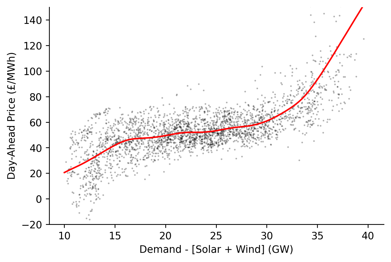
We'll then visualise the estimated fit alongside the historical observations
fig, ax = plt.subplots(dpi=250)

ax.plot(x_pred, y_pred, linewidth=1.5, color='r')
ax.scatter(s_dispatchable, s_price, color='k', s=0.5, alpha=0.25)

ax.set_ylim(-20, 150)
eda.hide_spines(ax)
ax.set_xlabel('Demand - [Solar + Wind] (GW)')
ax.set_ylabel('Day-Ahead Price (£/MWh)')
fig.savefig('../img/latest_gb_mcc.png', dpi=250)