Data Retrieval¶

This notebook outlines the retrieval of data from Electric Insights and Energy Charts using the moepy library. This data will be used in later user-guide notebooks.

Imports¶

from moepy import retrieval, eda

Electric Insights¶

To download data from all of the electric insights streams is as simple as calling get_EI_data and specifying the start and end dates. The data will be retrieved in 3 month batches as this is the maximum limit currently allowed by the API, you can change the freq parameter to adjust this.

Please save data once downloaded to avoid needless calls to the API.

start_date = '2010-01-01'
end_date = '2020-12-31'

df_EI = retrieval.get_EI_data(start_date, end_date)
df_EI.to_csv('../data/ug/electric_insights.csv')

df_EI.head()

100%|â–ˆâ–ˆâ–ˆâ–ˆâ–ˆâ–ˆâ–ˆâ–ˆâ–ˆâ–ˆâ–ˆâ–ˆâ–ˆâ–ˆâ–ˆâ–ˆâ–ˆâ–ˆâ–ˆâ–ˆâ–ˆâ–ˆâ–ˆâ–ˆâ–ˆâ–ˆâ–ˆâ–ˆâ–ˆâ–ˆâ–ˆâ–ˆâ–ˆâ–ˆâ–ˆâ–ˆâ–ˆâ–ˆâ–ˆâ–ˆâ–ˆâ–ˆâ–ˆâ–ˆâ–ˆâ–ˆâ–ˆâ–ˆâ–ˆâ–ˆâ–ˆâ–ˆâ–ˆâ–ˆâ–ˆâ–ˆâ–ˆâ–ˆâ–ˆâ–ˆâ–ˆâ–ˆâ–ˆâ–ˆâ–ˆâ–ˆâ–ˆâ–ˆâ–ˆâ–ˆâ–ˆâ–ˆâ–ˆâ–ˆâ–ˆâ–ˆâ–ˆâ–ˆâ–ˆâ–ˆâ–ˆâ–ˆ| 45/45 [08:51<00:00, 11.81s/it]

local_datetime	day_ahead_price	SP	imbalance_price	valueSum	temperature	TCO2_per_h	gCO2_per_kWh	nuclear	coal	...	demand	pumped_storage	wind_onshore	wind_offshore	french	irish
2010-01-01 00:00:00+00:00	32.91	1	55.77	55.77	1.1	16268	429	7.897	9.902	...	37.948	-0.435	None	None	1.963	-0.234
2010-01-01 00:30:00+00:00	33.25	2	59.89	59.89	1.1	16432	430	7.897	10.074	...	38.227	-0.348	None	None	1.974	-0.236
2010-01-01 01:00:00+00:00	32.07	3	53.15	53.15	1.1	16318	431	7.893	10.049	...	37.898	-0.424	None	None	1.983	-0.236
2010-01-01 01:30:00+00:00	31.99	4	38.48	38.48	1.1	15768	427	7.896	9.673	...	36.918	-0.575	None	None	1.983	-0.236
2010-01-01 02:00:00+00:00	31.47	5	37.7	37.7	1.1	15250	424	7.9	9.37	...	35.961	-0.643	None	None	1.983	-0.236

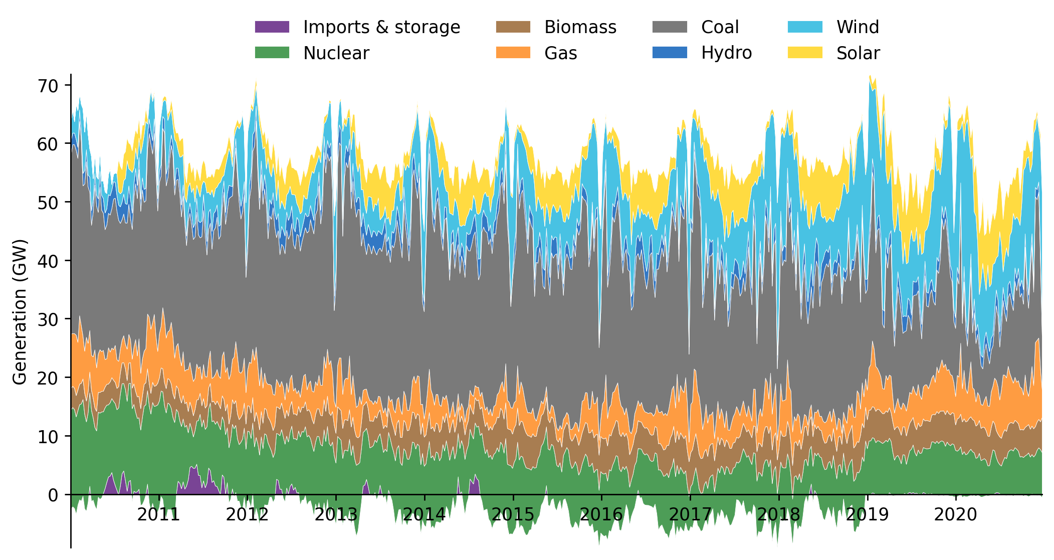
We'll visualise the time-series of output by fuel in the style of this paper, the author of which was also a creator of the Electric Insights site.

df_EI_plot = eda.clean_EI_df_for_plot(df_EI, freq='7D')

eda.stacked_fuel_plot(df_EI_plot, dpi=250)

<AxesSubplot:ylabel='Generation (GW)'>

png

Energy Charts¶

To download fuel generation data from the energy charts site call get_EC_data and specify the start and end dates.

As before, please save data once downloaded.

df_EC = retrieval.get_EC_data(start_date, end_date)

df_EC.head()

100%|â–ˆâ–ˆâ–ˆâ–ˆâ–ˆâ–ˆâ–ˆâ–ˆâ–ˆâ–ˆâ–ˆâ–ˆâ–ˆâ–ˆâ–ˆâ–ˆâ–ˆâ–ˆâ–ˆâ–ˆâ–ˆâ–ˆâ–ˆâ–ˆâ–ˆâ–ˆâ–ˆâ–ˆâ–ˆâ–ˆâ–ˆâ–ˆâ–ˆâ–ˆâ–ˆâ–ˆâ–ˆâ–ˆâ–ˆâ–ˆâ–ˆâ–ˆâ–ˆâ–ˆâ–ˆâ–ˆâ–ˆâ–ˆâ–ˆâ–ˆâ–ˆâ–ˆâ–ˆâ–ˆâ–ˆâ–ˆâ–ˆâ–ˆâ–ˆâ–ˆâ–ˆâ–ˆâ–ˆâ–ˆâ–ˆâ–ˆâ–ˆâ–ˆâ–ˆâ–ˆâ–ˆâ–ˆâ–ˆâ–ˆâ–ˆâ–ˆâ–ˆâ–ˆâ–ˆâ–ˆ| 576/576 [05:02<00:00,  1.91it/s]

local_datetime	Biomass	Brown Coal	Gas	Hard Coal	Hydro Power	Oil	Pumped Storage	Seasonal Storage	Uranium	Wind	Net Balance
2010-01-04 00:00:00+01:00	3.637	16.533	4.726	10.078	2.331	0	0.052	0.068	16.826	0.635	-1.229
2010-01-04 01:00:00+01:00	3.637	16.544	4.856	8.816	2.293	0	0.038	0.003	16.841	0.528	-1.593
2010-01-04 02:00:00+01:00	3.637	16.368	5.275	7.954	2.299	0	0.032	0	16.846	0.616	-1.378
2010-01-04 03:00:00+01:00	3.637	15.837	5.354	7.681	2.299	0	0.027	0	16.699	0.63	-1.624
2010-01-04 04:00:00+01:00	3.637	15.452	5.918	7.498	2.301	0.003	0.02	0	16.635	0.713	-0.731

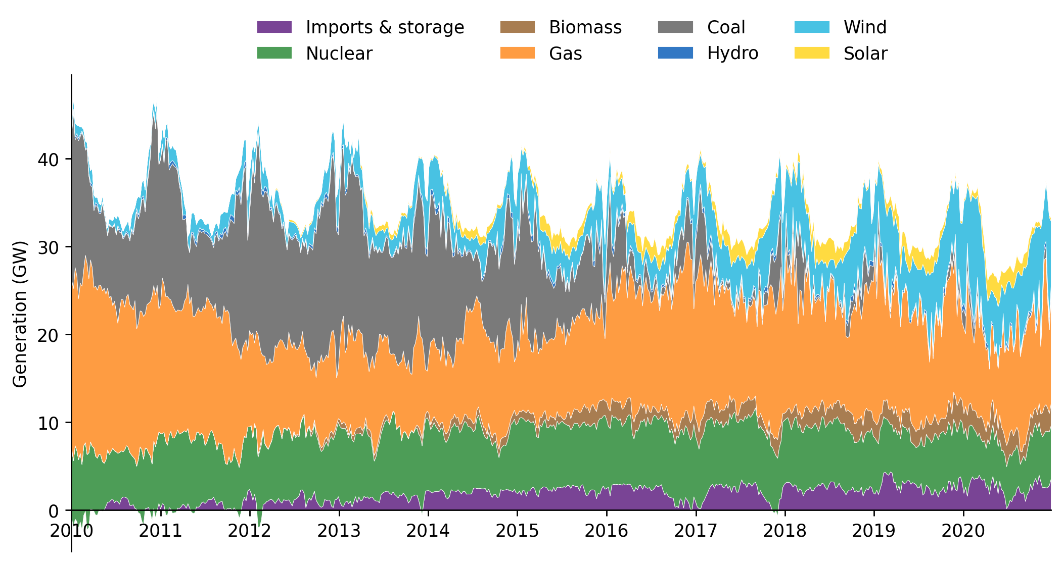
Once again we'll visualise the long-term average output time-series separated by fuel-type

df_EC_plot = eda.clean_EC_df_for_plot(df_EC)
eda.stacked_fuel_plot(df_EC_plot, dpi=250)

<AxesSubplot:ylabel='Generation (GW)'>

png