Quantile Estimation of Portugese Hydro Power Seasonality¶

In this example we'll use power output data from Portugese hydro-plants to demonstrate how the quantile LOWESS model can be used.

Imports¶

import pandas as pd

import matplotlib.pyplot as plt

from moepy import lowess, eda

Loading Data¶

We'll start by reading in the Portugese hydro output data

df_portugal_hydro = pd.read_csv('../data/lowess_examples/portugese_hydro.csv')

df_portugal_hydro.index = pd.to_datetime(df_portugal_hydro['datetime'])
df_portugal_hydro = df_portugal_hydro.drop(columns='datetime')

df_portugal_hydro['day_of_the_year'] = df_portugal_hydro.index.dayofyear
df_portugal_hydro = df_portugal_hydro.resample('D').mean()
df_portugal_hydro = df_portugal_hydro.rename(columns={'power_MW': 'average_power_MW'})

df_portugal_hydro.head()

datetime	average_power_MW	day_of_the_year
2015-01-01	698.5	1
2015-01-02	1065.75	2
2015-01-03	905.125	3
2015-01-04	795.708	4
2015-01-05	1141.62	5

Quantile LOWESS¶

We now just need to feed this data into our quantile_model wrapper

# Estimating the quantiles
df_quantiles = lowess.quantile_model(df_portugal_hydro['day_of_the_year'].values,
                                     df_portugal_hydro['average_power_MW'].values,
                                     frac=0.4, num_fits=40)

# Cleaning names and sorting for plotting
df_quantiles.columns = [f'p{int(col*100)}' for col in df_quantiles.columns]
df_quantiles = df_quantiles[df_quantiles.columns[::-1]]

df_quantiles.head()

100% 9/9 [00:16<00:02, 1.73s/it]

x	p90	p80	p70	p60	p50	p40	p30	p20	p10
1	1885.08	1400.78	1006.97	910.769	795.475	693.001	604.221	498.096	407.17
2	1885.93	1406.29	1015.76	917.074	800.255	697.121	607.521	500.673	409.021
3	1886.8	1411.81	1024.54	923.37	805.008	701.225	610.814	503.239	410.866
4	1887.68	1417.32	1033.31	929.659	809.738	705.317	614.105	505.797	412.695
5	1888.57	1422.84	1042.08	935.952	814.456	709.409	617.404	508.359	414.485

We can then visualise the estimated quantile fits of the data

fig, ax = plt.subplots(dpi=150)

ax.scatter(df_portugal_hydro['day_of_the_year'], df_portugal_hydro['average_power_MW'], s=1, color='k', alpha=0.5)
df_quantiles.plot(cmap='viridis', legend=False, ax=ax)

eda.hide_spines(ax)
ax.legend(frameon=False, bbox_to_anchor=(1, 0.8))
ax.set_xlabel('Day of the Year')
ax.set_ylabel('Hydro Power Average (MW)')
ax.set_xlim(0, 365)
ax.set_ylim(0)

(0.0, 2620.8375)

png

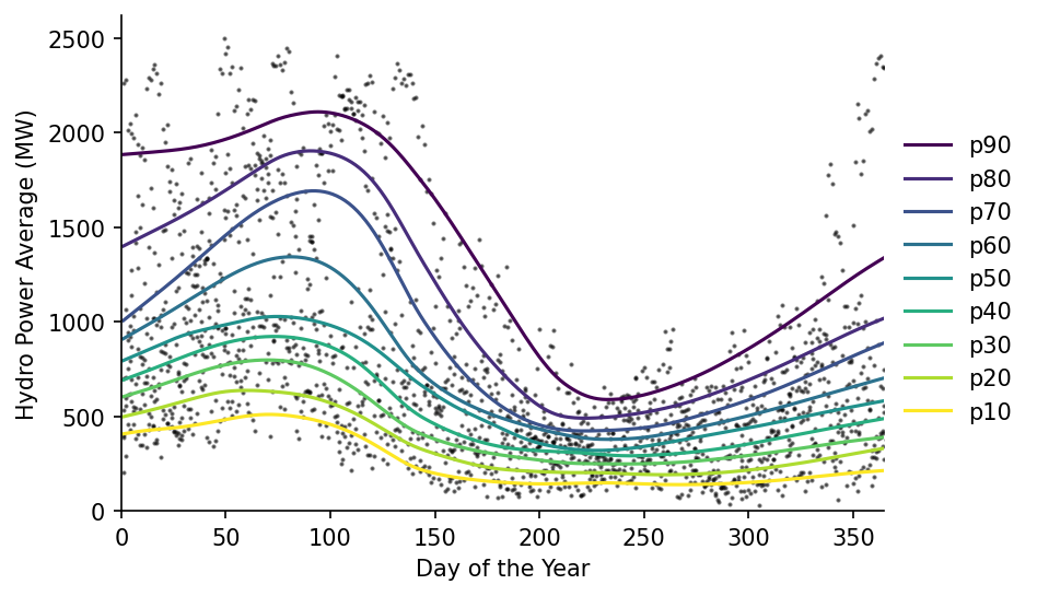
We can also ask questions like: "what day of a standard year would the lowest power output be recorded?"

scenario = 'p50'

print(f'In a {scenario} year the lowest hydro power output will most likely fall on day {df_quantiles[scenario].idxmin()}')

In a p50 year the lowest hydro power output will most likely fall on day 228

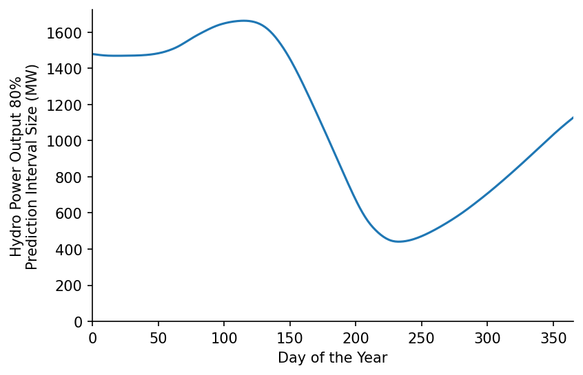
We can also identify the peridos when our predictions will have the greatest uncertainty

s_80pct_pred_intvl = df_quantiles['p90'] - df_quantiles['p10']

print(f'Day {s_80pct_pred_intvl.idxmax()} is most likely to have the greatest variation in hydro power output')

# Plotting
fig, ax = plt.subplots(dpi=150)

s_80pct_pred_intvl.plot(ax=ax)

eda.hide_spines(ax)
ax.set_xlabel('Day of the Year')
ax.set_ylabel('Hydro Power Output 80%\nPrediction Interval Size (MW)')
ax.set_xlim(0, 365)
ax.set_ylim(0)

Day 115 is most likely to have the greatest variation in hydro power output





(0.0, 1724.0724938300584)

png