Tables & Figures Generation
![]()
This notebook provides a programmatic workflow for generating the tables used in the MOE paper, as well as the diagram to show the time-adaptive smoothing weights.
Imports
import json
import numpy as np
import pandas as pd

import seaborn as sns
import matplotlib.pyplot as plt

from IPython.display import Latex, JSON

from moepy import eda, lowess
Tables
Power Systems Overview
We'll first load in the DE data
df_DE = eda.load_DE_df('../data/raw/energy_charts.csv', '../data/raw/ENTSOE_DE_price.csv')

df_DE.head()
| local_datetime | Biomass | Brown Coal | Gas | Hard Coal | Hydro Power | Oil | Others | Pumped Storage | Seasonal Storage | Solar | Uranium | Wind | Net Balance | demand | price |
|---|---|---|---|---|---|---|---|---|---|---|---|---|---|---|---|
| 2010-01-03 23:00:00+00:00 | 3.637 | 16.533 | 4.726 | 10.078 | 2.331 | 0 | 0 | 0.052 | 0.068 | 0 | 16.826 | 0.635 | -1.229 | 53.657 | nan |
| 2010-01-04 00:00:00+00:00 | 3.637 | 16.544 | 4.856 | 8.816 | 2.293 | 0 | 0 | 0.038 | 0.003 | 0 | 16.841 | 0.528 | -1.593 | 51.963 | nan |
| 2010-01-04 01:00:00+00:00 | 3.637 | 16.368 | 5.275 | 7.954 | 2.299 | 0 | 0 | 0.032 | 0 | 0 | 16.846 | 0.616 | -1.378 | 51.649 | nan |
| 2010-01-04 02:00:00+00:00 | 3.637 | 15.837 | 5.354 | 7.681 | 2.299 | 0 | 0 | 0.027 | 0 | 0 | 16.699 | 0.63 | -1.624 | 50.54 | nan |
| 2010-01-04 03:00:00+00:00 | 3.637 | 15.452 | 5.918 | 7.498 | 2.301 | 0.003 | 0 | 0.02 | 0 | 0 | 16.635 | 0.713 | -0.731 | 51.446 | nan |
Clean it up then calculate the relevant summary statistics
year = '2019'

s_DE_RES_output = df_DE[['Wind', 'Solar']].sum(axis=1)
s_DE_demand = df_DE['demand']
s_DE_price = df_DE['price']

s_DE_RES_pct = s_DE_RES_output/s_DE_demand

DE_annual_RES_pct = s_DE_RES_pct[year].mean()
DE_annual_demand_avg = s_DE_demand[year].mean()
DE_annual_price_avg = s_DE_price[year].mean()
DE_annual_price_min = s_DE_price[year].min()
DE_annual_price_max = s_DE_price[year].max()

DE_annual_RES_pct, DE_annual_demand_avg, DE_annual_price_avg
(0.325151836935705, 59.04589823059361, 37.668148401826485)
We'll also estimate the carbon intensity
DE_fuel_to_co2_intensity = {
    'Biomass': 0.39,
    'Brown Coal': 0.36,
    'Gas': 0.23,
    'Hard Coal': 0.34,
    'Hydro Power': 0,
    'Oil': 0.28,
    'Others': 0,
    'Pumped Storage': 0,
    'Seasonal Storage': 0,
    'Solar': 0,
    'Uranium': 0,
    'Wind': 0,
    'Net Balance': 0
}

s_DE_emissions_tonnes = (df_DE
                         [DE_fuel_to_co2_intensity.keys()]
                         .multiply(1e3) # converting to MWh
                         .multiply(DE_fuel_to_co2_intensity.values())
                         .sum(axis=1)
                        )

s_DE_emissions_tonnes = s_DE_emissions_tonnes[s_DE_emissions_tonnes>2000]
s_DE_carbon_intensity = s_DE_emissions_tonnes/s_DE_demand.loc[s_DE_emissions_tonnes.index]

DE_annual_emissions_tonnes = s_DE_emissions_tonnes[year].mean()
DE_annual_ci_avg = s_DE_carbon_intensity[year].mean()

DE_annual_emissions_tonnes, DE_annual_ci_avg
(9496.454279394979, 163.22025761797656)
We'll do the same for GB
# Loading in
df_EI = pd.read_csv('../data/raw/electric_insights.csv')

df_EI = df_EI.set_index('local_datetime')
df_EI.index = pd.to_datetime(df_EI.index, utc=True)

# Extracting RES, demand, and price series
s_GB_RES = df_EI[['wind', 'solar']].sum(axis=1)
s_GB_demand = df_EI['demand']
s_GB_price = df_EI['day_ahead_price']

# Generating carbon intensity series
GB_fuel_to_co2_intensity = {
    'nuclear': 0,
    'biomass': 0.121, # from EI
    'coal': 0.921, # DUKES 2018 value
    'gas': 0.377, # DUKES 2018 value (lower than many CCGT estimates, let alone OCGT)
    'hydro': 0,
    'pumped_storage': 0,
    'solar': 0,
    'wind': 0,
    'belgian': 0.4,
    'dutch': 0.474, # from EI
    'french': 0.053, # from EI
    'ireland': 0.458, # from EI
    'northern_ireland': 0.458 # from EI
}

s_GB_emissions_tonnes = (df_EI
                         [GB_fuel_to_co2_intensity.keys()]
                         .multiply(1e3*0.5) # converting to MWh
                         .multiply(GB_fuel_to_co2_intensity.values())
                         .sum(axis=1)
                        )

s_GB_emissions_tonnes = s_GB_emissions_tonnes[s_GB_emissions_tonnes>2000]
s_GB_carbon_intensity = s_GB_emissions_tonnes/s_GB_demand.loc[s_GB_emissions_tonnes.index]

# Calculating annual averages
GB_annual_emissions_tonnes = s_GB_emissions_tonnes[year].mean()
GB_annual_ci_avg = s_GB_carbon_intensity[year].mean()
GB_annual_RES_pct = (s_GB_RES[year]/s_GB_demand[year]).mean()
GB_annual_demand_avg = s_GB_demand[year].mean()
GB_annual_price_avg = s_GB_price[year].mean()
GB_annual_price_min = s_GB_price[year].min()
GB_annual_price_max = s_GB_price[year].max()
Then combine the results in a single table
system_overview_data = {
    'Germany': {
        'Average Solar/Wind Generation (%)': round(100*DE_annual_RES_pct, 2),
        'Average Demand (GW)': round(DE_annual_demand_avg, 2),
        'Average Price ([EUR,GBP]/MWh)': round(DE_annual_price_avg, 2),
        'Minimum Price ([EUR,GBP]/MWh)': round(DE_annual_price_min, 2),
        'Maximum Price ([EUR,GBP]/MWh)': round(DE_annual_price_max, 2),
        'Average Carbon Intensity  (gCO2/kWh)': round(DE_annual_ci_avg, 2),
    },
    'Great Britain': {
        'Average Solar/Wind Generation (%)': round(100*GB_annual_RES_pct, 2),
        'Average Demand (GW)': round(GB_annual_demand_avg, 2),
        'Average Price ([EUR,GBP]/MWh)': round(GB_annual_price_avg, 2),
        'Minimum Price ([EUR,GBP]/MWh)': round(GB_annual_price_min, 2),
        'Maximum Price ([EUR,GBP]/MWh)': round(GB_annual_price_max, 2),
        'Average Carbon Intensity  (gCO2/kWh)': round(GB_annual_ci_avg, 2),
    }
}

df_system_overview = pd.DataFrame(system_overview_data)

df_system_overview.head()
| Unnamed: 0 | Germany | Great Britain |
|---|---|---|
| Average Solar/Wind Generation (%) | 32.52 | 24.71 |
| Average Demand (GW) | 59.05 | 32.58 |
| Average Price ([EUR,GBP]/MWh) | 37.67 | 41.81 |
| Minimum Price ([EUR,GBP]/MWh) | -90.01 | -72.84 |
| Maximum Price ([EUR,GBP]/MWh) | 121.46 | 152 |
Which we'll then output as a LaTeX table
get_lined_column_format = lambda n_cols:''.join(n_cols*['|l']) + '|'

caption = f'Markets overview for {year}'
label = 'table:overview_table'
column_format = get_lined_column_format(df_system_overview.shape[1]+1)

latex_str = df_system_overview.to_latex(column_format=column_format, caption=caption, label=label)

latex_replacements = {
    'CO2': 'CO\\textsubscript{2}',
    '\\\\\n': '\\\\ \\midrule\n',
    'midrule': 'hline',
    'toprule': 'hline',
    'bottomrule': '',
    '\n\\\n': '\n',
    '\\hline\n\\hline': '\\hline'
}

for old, new in latex_replacements.items():
    latex_str = latex_str.replace(old, new)

Latex(latex_str)
Carbon Intensity Estimates
We'll clean up our GB carbon intensity estimates
def clean_idxs(s):
    s.index = s.index.str.replace('_', ' ').str.title()
    return s

df_GB_non0_co2_intensity = (pd
                            .Series(GB_fuel_to_co2_intensity)
                            .replace(0, np.nan)
                            .dropna()
                            .drop(['belgian', 'northern_ireland'])
                            .pipe(clean_idxs)
                            .multiply(1e3)
                            .astype(int)
                            .to_frame()
                            .T
                            .rename({0: 'gCO2/kWh'})
                           )

df_GB_non0_co2_intensity
| Unnamed: 0 | Biomass | Coal | Gas | Dutch | French | Ireland |
|---|---|---|---|---|---|---|
| gCO2/kWh | 121 | 921 | 377 | 474 | 53 | 458 |
And output them as a LaTeX table
caption = 'Carbon intensity factors for fuel-types and interconnection on the GB power system'
label = 'table:GB_co2_intensity_table'
column_format = get_lined_column_format(df_GB_non0_co2_intensity.shape[1]+1)

latex_str = df_GB_non0_co2_intensity.to_latex(column_format=column_format, caption=caption, label=label)

latex_replacements = {
    'CO2': 'CO\\textsubscript{2}',
    '\\\\\n': '\\\\ \\midrule\n',
    'midrule': 'hline',
    'toprule': 'hline',
    'bottomrule': '',
    '\n\\\n': '\n',
    '\\hline\n\\hline': '\\hline'
}

for old, new in latex_replacements.items():
    latex_str = latex_str.replace(old, new)

Latex(latex_str)
We'll then do the same for DE
df_DE_non0_co2_intensity = (pd
                            .Series(DE_fuel_to_co2_intensity)
                            .replace(0, np.nan)
                            .dropna()
                            [['Biomass', 'Brown Coal', 'Hard Coal', 'Gas', 'Oil']]
                            .pipe(clean_idxs)
                            .multiply(1e3)
                            .astype(int)
                            .to_frame()
                            .T
                            .rename({0: 'gCO2/kWh'})
                           )

df_DE_non0_co2_intensity
| Unnamed: 0 | Biomass | Brown Coal | Hard Coal | Gas | Oil |
|---|---|---|---|---|---|
| gCO2/kWh | 390 | 360 | 340 | 230 | 280 |
caption = 'Carbon intensity factors for fuel-types and interconnection on the DE power system'
label = 'table:DE_co2_intensity_table'
column_format = get_lined_column_format(df_DE_non0_co2_intensity.shape[1]+1)

latex_str = df_DE_non0_co2_intensity.to_latex(column_format=column_format, caption=caption, label=label)

for old, new in latex_replacements.items():
    latex_str = latex_str.replace(old, new)

Latex(latex_str)
Electricity Price Forecasting Metrics
We'll start by loading in our previously saved model metrics
with open('../data/results/price_model_accuracy_metrics.json', 'r') as fp:
    model_accuracy_metrics = json.load(fp)

JSON(model_accuracy_metrics)
<IPython.core.display.JSON object>
We'll parse the MAE results into a new table
model_accuracy_data = {
    'Germany': {
        'Dispatchable Load': round(model_accuracy_metrics['DE_dispatch']['mean_abs_err'], 2),
        'Total Load': round(model_accuracy_metrics['DE_demand']['mean_abs_err'], 2),
    },
    'Great Britain': {
        'Dispatchable Load': round(model_accuracy_metrics['GB_dispatch']['mean_abs_err'], 2),
        'Total Load': round(model_accuracy_metrics['GB_demand']['mean_abs_err'], 2),
    }
}

df_model_accuracy = pd.DataFrame(model_accuracy_data).T

df_model_accuracy.head()
| Unnamed: 0 | Dispatchable Load | Total Load |
|---|---|---|
| Germany | 5.85 | 18.28 |
| Great Britain | 6.56 | 8.42 |
Which we'll output as a LaTeX table
caption = 'Price forecasting model accuracy when regressing against dispatchable and total load for GB and DE.'
label = 'table:model_accuracy_table'
column_format = get_lined_column_format(df_model_accuracy.shape[1]+1)

latex_str = df_model_accuracy.to_latex(column_format=column_format, caption=caption, label=label)

for old, new in latex_replacements.items():
    latex_str = latex_str.replace(old, new)

Latex(latex_str)
Price and CO2 MOE Results
We'll first load in all of the price and carbon MOE time-series
def set_dt_idx(df, dt_idx_col='local_datetime'):
    df = df.set_index(dt_idx_col)
    df.index = pd.to_datetime(df.index, utc=True)

    return df

df_GB_price_results_ts = pd.read_csv('../data/results/GB_price.csv').pipe(set_dt_idx)
df_DE_price_results_ts = pd.read_csv('../data/results/DE_price.csv').pipe(set_dt_idx)
df_GB_carbon_results_ts = pd.read_csv('../data/results/GB_carbon.csv').pipe(set_dt_idx)
df_DE_carbon_results_ts = pd.read_csv('../data/results/DE_carbon.csv').pipe(set_dt_idx)

df_GB_price_results_ts.head()
| local_datetime | prediction | counterfactual | observed | moe |
|---|---|---|---|---|
| 2009-01-01 00:00:00+00:00 | 37.2034 | 37.3134 | 58.05 | 0.109938 |
| 2009-01-01 00:30:00+00:00 | 37.3134 | 37.5351 | 56.33 | 0.221756 |
| 2009-01-01 01:00:00+00:00 | 36.7685 | 36.9851 | 52.98 | 0.216574 |
| 2009-01-01 01:30:00+00:00 | 35.5952 | 35.8076 | 50.39 | 0.212469 |
| 2009-01-01 02:00:00+00:00 | 34.8494 | 35.0631 | 48.7 | 0.213697 |
We'll then calculate their summary statistics
MOE_results_data = {
    'Germany': {
        'Price ([EUR,GBP]/MWh)': round(df_DE_price_results_ts.loc[year, 'moe'].mean(), 2),
        'Price Reduction (%)': round(100*(df_DE_price_results_ts.loc[year, 'moe']*df_DE['demand']).sum()/((df_DE_price_results_ts.loc[year, 'observed']+df_DE_price_results_ts.loc[year, 'moe'])*df_DE['demand']).sum(), 2),
        'Carbon (Tonnes/h)': round(df_DE_carbon_results_ts.loc[year, 'moe'].mean(), 2),
        'Carbon Reduction (%)': round(100*(df_DE_carbon_results_ts.loc[year, 'moe'].sum()/(df_DE_carbon_results_ts.loc[year, 'observed']+df_DE_carbon_results_ts.loc[year, 'moe']).sum()).mean(), 2)
    },
    'Great Britain': {
        'Price ([EUR,GBP]/MWh)': round(df_GB_price_results_ts.loc[year, 'moe'].mean(), 2),
        'Price Reduction (%)': round(100*(df_GB_price_results_ts.loc[year, 'moe']*df_EI['demand']).sum()/((df_GB_price_results_ts.loc[year, 'observed']+df_GB_price_results_ts.loc[year, 'moe'])*df_EI['demand']).sum(), 2),
        'Carbon (Tonnes/h)': round(df_GB_carbon_results_ts.loc[year, 'moe'].mean(), 2), # doubled to make it the same hourly rate as DE
        'Carbon Reduction (%)': round(100*(df_GB_carbon_results_ts.loc[year, 'moe'].sum()/(df_GB_carbon_results_ts.loc[year, 'observed']+df_GB_carbon_results_ts.loc[year, 'moe']).sum()).mean(), 2)
    }
}

df_MOE_results = (pd
                  .DataFrame(MOE_results_data)
                 )

df_MOE_results.head()
| Unnamed: 0 | Germany | Great Britain |
|---|---|---|
| Price ([EUR,GBP]/MWh) | 20.53 | 9.8 |
| Price Reduction (%) | 36.7 | 19.3 |
| Carbon (Tonnes/h) | 5085.92 | 1637.2 |
| Carbon Reduction (%) | 34.88 | 33.53 |
And export the output as a LaTeX table
caption = f'Merit Order Effect results overview for {year} (weighted by volume). Price reduction is expressed in terms of the percentage decrease relative to the counter-factual price that would have occurred with RES generation'
label = 'table:moe_results_table'
column_format = get_lined_column_format(df_MOE_results.shape[1]+1)

latex_str = df_MOE_results.to_latex(column_format=column_format, caption=caption, label=label)

for old, new in latex_replacements.items():
    latex_str = latex_str.replace(old, new)

Latex(latex_str)
Literature Review
Lastly we'll create our largest table, containing results from across the literature
lit_results_data = [
    {
        'Study': 'Sensfuss et al. (2008)',
        'MOE': '7.83 €/MWh',
        'Period': '2006',
        'Region': 'Germany',
        'Method': 'ESS',
    },
    {
        'Study': 'Weigt (2009)',
        'MOE': '10 €/MWh',
        'Period': '2006-2008',
        'Region': 'Germany',
        'Method': 'ESS',
    },
    {
        'Study': 'Keles et al. (2013)',
        'MOE': '5.90 €/MWh',
        'Period': '2006–2009',
        'Region': 'Germany',
        'Method': 'RPR',
    },
    {
        'Study': 'Mulder and Scholtens (2013)',
        'MOE': '0.03% (per p.p increase in wind speeds)',
        'Period': '2006–2011',
        'Region': 'Germany',
        'Method': 'RPR',
    },
    {
        'Study': 'Tveten et al. (2013)',
        'MOE': '5.25 €/MWh (solar)',
        'Period': '2006-2011',
        'Region': 'Germany',
        'Method': 'RPR',
    },
    {
        'Study': 'Wurzburg et al. (2013)',
        'MOE': '2%',
        'Period': '2010-2012',
        'Region': 'Germany & Austria',
        'Method': 'RPR',
    },
    {
        'Study': 'Cludius et al. (2014)',
        'MOE': '8 €/MWh',
        'Period': '2010-2012',
        'Region': 'Germany',
        'Method': 'RPR',
    },
    {
        'Study': 'Ketterer (2014)',
        'MOE': '1.46% (per p.p increase in wind generation)',
        'Period': '2012',
        'Region': 'Germany',
        'Method': 'RPR',
    },
    {
        'Study': 'Ederer (2015)',
        'MOE': '1.3% (per annual TWh of wind)',
        'Period': '2006-2014',
        'Region': 'Germany',
        'Method': 'MSS',
    },
#     {
#         'Study': 'Kyritsis et al. (2017)',
#         'MOE': '-',
#         'Period': '2010-2015',
#         'Region': 'Germany',
#         'Method': 'RPR',
#     },
    {
        'Study': 'Bublitz et al. (2017)',
        'MOE': '5.40 €/MWh',
        'Period': '2011-2015',
        'Region': 'Germany',
        'Method': 'ESS',
    },
    {
        'Study': 'Bublitz et al. (2017)',
        'MOE': '6.80 €/MWh',
        'Period': '2011-2015',
        'Region': 'Germany',
        'Method': 'RPR',
    },
    {
        'Study': 'de Miera et al. (2008)',
        'MOE': '25.1%',
        'Period': '2007',
        'Region': 'Spain',
        'Method': 'ESS',
    },
    {
        'Study': 'Gelabert et al. (2011)',
        'MOE': '3.7%',
        'Period': '2005-2012',
        'Region': 'Spain',
        'Method': 'RPR',
    },
    {
        'Study': 'Ciarreta et al. (2014)',
        'MOE': '45 €/MWh',
        'Period': '2012',
        'Region': 'Spain',
        'Method': 'ESS',
    },
    {
        'Study': 'Clo et al. (2015)',
        'MOE': '2.3 €/MWh (solar), 4.2 €/MWh (wind)',
        'Period': '2005–2013',
        'Region': 'Italy',
        'Method': 'RPR',
    },
    {
        'Study': 'Munksgaard and Morthorst (2008)',
        'MOE': '4 €/MWh',
        'Period': '2006',
        'Region': 'Denmark',
        'Method': 'RPR',
    },
#     {
#         'Study': 'Jonsson et al. (2010)',
#         'MOE': '-',
#         'Period': '2006-2007',
#         'Region': 'Denmark',
#         'Method': 'RPR',
#     },
    {
        'Study': 'Denny et al. (2017)',
        'MOE': '3.40 €/MWh (per GWh of wind)',
        'Period': '2009',
        'Region': 'Ireland',
        'Method': 'RPR',
    },
    {
        'Study': 'Lunackova et al. (2017)',
        'MOE': '1.2% (per 10% increase in RES)',
        'Period': '2010-2015',
        'Region': 'Czech Republic',
        'Method': 'RPR',
    },
    {
        'Study': 'Dillig et al. (2016)',
        'MOE': '50.29 €/MWh',
        'Period': '2011-2013',
        'Region': 'Germany',
        'Method': 'MSS',
    },
    {
        'Study': 'McConnell et al. (2013)',
        'MOE': '8.6%',
        'Period': '2009-2010',
        'Region': 'Australia',
        'Method': 'MSS',
    },
    {
        'Study': 'Moreno et al. (2012)',
        'MOE': '-0.018% (per p.p. increase in RES)',
        'Period': '1998–2009',
        'Region': 'EU-27',
        'Method': 'RPR',
    },
    {
        'Study': 'Woo et al. (2011)',
        'MOE': '1.53 $/MWh',
        'Period': '2010',
        'Region': 'Texas',
        'Method': 'RPR',
    },
    {
        'Study': 'Kaufmann and Vaid (2016)',
        'MOE': '1.86 $/MWh (solar)',
        'Period': '2012',
        'Region': 'Massachusetts',
        'Method': 'RPR',
    },
    {
        'Study': 'Woo et al. (2016)',
        'MOE': '5.3 $/MWh (solar) and 3.3 $/MWh (wind) per GWh of RES',
        'Period': '2012-2015',
        'Region': 'California',
        'Method': 'RPR',
    },
    {
        'Study': 'Paraschiv et al. (2014)',
        'MOE': '0.15% (per MWh of RES)',
        'Period': '2010-2013',
        'Region': 'Germany',
        'Method': 'RPR',
    },
    {
        'Study': 'O\'Mahoney and Denny (2011)',
        'MOE': '12%',
        'Period': '2009',
        'Region': 'Ireland',
        'Method': 'RPR',
    },
    {
        'Study': 'Hildmann et al. (2015)',
        'MOE': '18.6 €/MWh',
        'Period': '2013',
        'Region': 'Germany and Austria',
        'Method': 'MSS',
    },
    {
        'Study': 'Gil et al. (2012)',
        'MOE': '9.72 €/MWh',
        'Period': '2007-2010',
        'Region': 'Spain',
        'Method': 'RPR',
    },
#     { # Removed due to language barrier preventing method from being discerned
#         'Study': 'Weber and Woll (2007)',
#         'MOE': '4 €/MWh',
#         'Period': '2006',
#         'Region': 'Germany',
#         'Method': '-',
#     },
    {
        'Study': 'Halttunen et al. (2021)',
        'MOE': '0.631 €/MWh (per p.p. increase in RES)',
        'Period': '2012-2019',
        'Region': 'Germany',
        'Method': 'RPR',
    },
    {
        'Study': 'Halttunen et al. (2021)',
        'MOE': '0.482 €/MWh (per p.p. increase in RES)',
        'Period': '2010-2019',
        'Region': 'Germany',
        'Method': 'RPR',
    }
]

df_lit_results = pd.DataFrame(lit_results_data)

df_lit_results['Study Year'] = df_lit_results['Study'].str.split('(').str[1].str.replace(')', '').astype(int)
df_lit_results = df_lit_results.sort_values(['Method', 'Study Year', 'Study']).drop(columns=['Study Year']).reset_index(drop=True)

df_lit_results.head()
<ipython-input-35-79dbc1b60908>:237: FutureWarning: The default value of regex will change from True to False in a future version. In addition, single character regular expressions will*not* be treated as literal strings when regex=True.
  df_lit_results['Study Year'] = df_lit_results['Study'].str.split('(').str[1].str.replace(')', '').astype(int)
| Unnamed: 0 | Study | MOE | Period | Region | Method |
|---|---|---|---|---|---|
| 0 | Sensfuss et al. (2008) | 7.83 €/MWh | 2006 | Germany | ESS |
| 1 | de Miera et al. (2008) | 25.1% | 2007 | Spain | ESS |
| 2 | Weigt (2009) | 10 €/MWh | 2006-2008 | Germany | ESS |
| 3 | Ciarreta et al. (2014) | 45 €/MWh | 2012 | Spain | ESS |
| 4 | Bublitz et al. (2017) | 5.40 €/MWh | 2011-2015 | Germany | ESS |
We'll also export this as a LaTeX table
caption = 'Results overview from the MOE literature. All MOE percentages are expressed in terms of the reduction in prices relative to if renewables had not been present on the system.'
label = 'table:lit_results_table'
column_format = get_lined_column_format(df_lit_results.shape[1]+1)

latex_str = df_lit_results.to_latex(column_format=column_format, caption=caption, label=label, index=False)

for old, new in latex_replacements.items():
    latex_str = latex_str.replace(old, new)

Latex(latex_str)
Figures
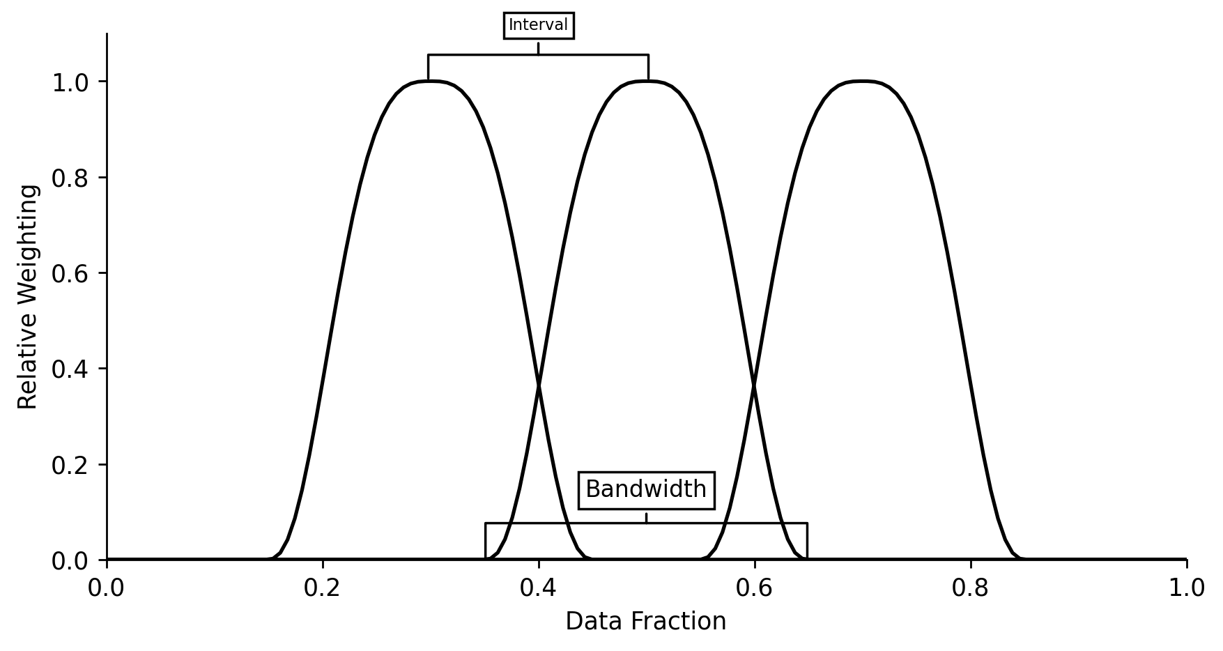
Time Dimension Hyper-Parameters
We'll create a plot showing an example of how regression dates are converted into weightings for the time-series
x = np.linspace(0, 1, 150)
centers = [0.3, 0.5, 0.7]

# Plotting
fig, ax = plt.subplots(dpi=250, figsize=(8, 4))

for center in centers:
    dist = lowess.get_dist(x, center)
    dist_threshold = lowess.get_dist_threshold(dist, frac=0.3)
    weights = lowess.dist_to_weights(dist, dist_threshold)

    ax.plot(x, weights, color='k')

x_pos = 0.4
ax.annotate('Interval', xy=(x_pos, 0.95), xytext=(x_pos, 1.00), xycoords='axes fraction',
            fontsize=6.5, ha='center', va='bottom',
            bbox=dict(boxstyle='square', fc='white'),
            arrowprops=dict(arrowstyle='-[, widthB=7.0, lengthB=1.5', lw=1.0))

x_pos = 0.5
ax.annotate('Bandwidth', xy=(x_pos, 0.06), xytext=(x_pos, 0.11), xycoords='axes fraction',
            fontsize=9.5, ha='center', va='bottom',
            bbox=dict(boxstyle='square', fc='white'),
            arrowprops=dict(arrowstyle='-[, widthB=7.0, lengthB=1.5', lw=1.0))

ax.set_xlim(0, 1)
ax.set_ylim(0, 1.1)
eda.hide_spines(ax)
ax.set_xlabel('Data Fraction')
ax.set_ylabel('Relative Weighting')
Text(0, 0.5, 'Relative Weighting')
Merit Order Effect Diagram
We'll start by pre-processing the data and filtering for the 16/17 winter
df_EI_model = df_EI.loc['2016-12':'2017-01', ['day_ahead_price', 'demand', 'solar', 'wind']].dropna()

s_demand = df_EI_model['demand']
s_price = df_EI_model['day_ahead_price']
s_dispatchable = df_EI_model['demand'] - df_EI_model[['solar', 'wind']].sum(axis=1)
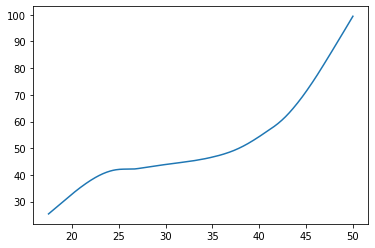
We'll now fit our model
x_pred = np.linspace(17.5, 50, 326)

y_pred = lowess.lowess_fit_and_predict(s_dispatchable.values,
                                       s_price.values,
                                       frac=0.3,
                                       num_fits=30,
                                       x_pred=x_pred)

s_pred = pd.Series(y_pred, index=x_pred)
s_pred.index = pd.Series(s_pred.index).round(1).values

s_pred.plot()
<AxesSubplot:>
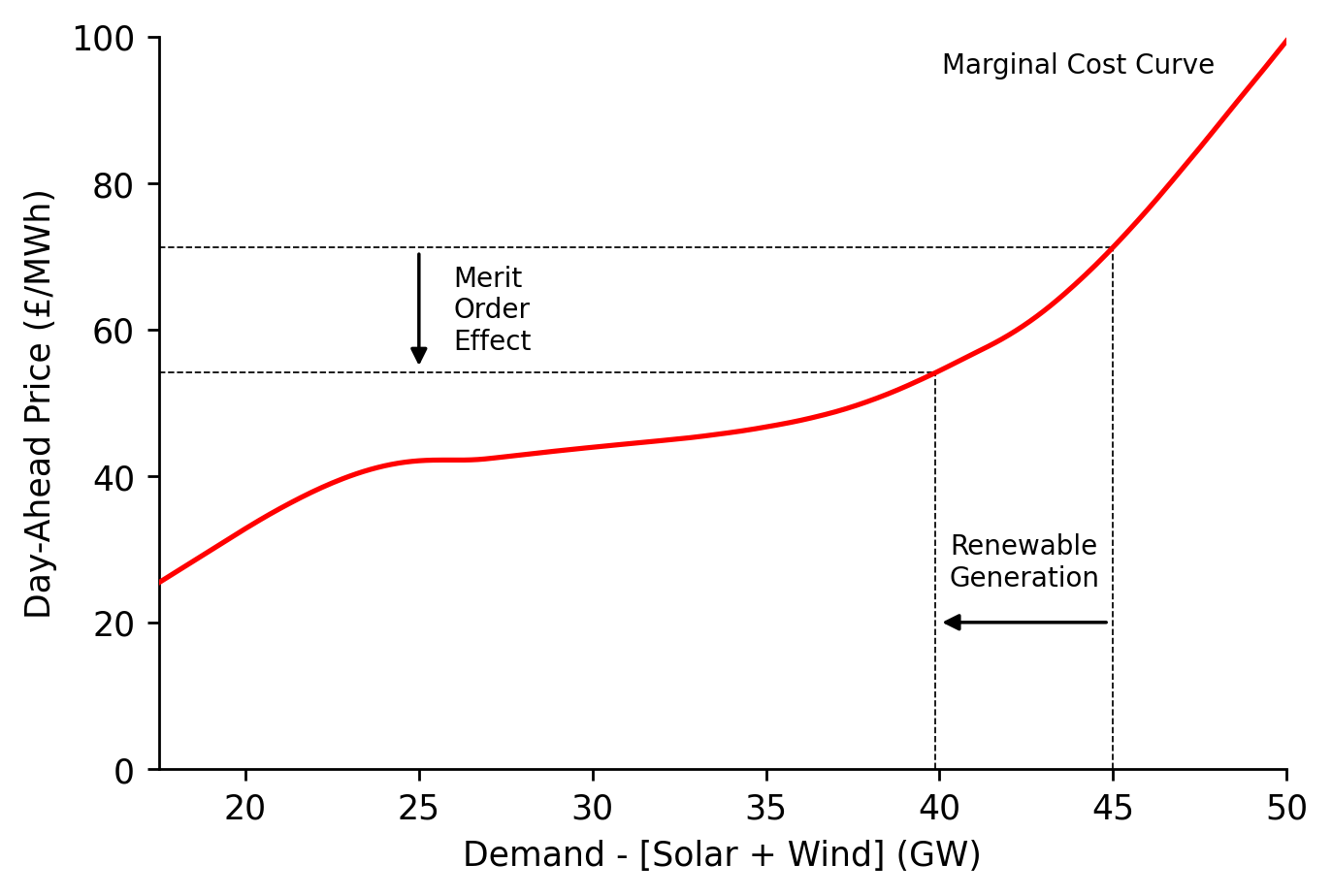
Next we can simulate how the price would change from a demand of 45 GW using the average RES output
residual_demand_without_RES =  45
residual_demand_with_RES = residual_demand_without_RES - (s_demand-s_dispatchable).mean()

price_with_RES = s_pred.loc[round(residual_demand_with_RES, 1)]
price_without_RES = s_pred.loc[round(residual_demand_without_RES, 1)]

round(price_with_RES, 2), round(price_without_RES, 2)
(54.13, 71.22)
We're now ready to plot how the intersection between supply and residual demand changes, with annotations explaining the drivers and effects
ylim = (0, 100)
xlim = (17.5, 50)
intersection_linestyle = 'k--'
linewidth = 0.5

# Plotting
fig, ax = plt.subplots(dpi=250)

s_pred.plot(linewidth=1.5, color='r', ax=ax, zorder=3)
ax.plot([residual_demand_without_RES, residual_demand_without_RES], [ylim[0], price_without_RES], intersection_linestyle, linewidth=linewidth)
ax.plot([residual_demand_with_RES, residual_demand_with_RES], [ylim[0], price_with_RES], intersection_linestyle, linewidth=linewidth)
ax.plot([xlim[0], residual_demand_without_RES], [price_without_RES, price_without_RES], intersection_linestyle, linewidth=linewidth)
ax.plot([xlim[0], residual_demand_with_RES], [price_with_RES, price_with_RES], intersection_linestyle, linewidth=linewidth)

ax.set_xlim(*xlim)
ax.set_ylim(*ylim)
eda.hide_spines(ax)
ax.set_xlabel('Demand - [Solar + Wind] (GW)')
ax.set_ylabel('Day-Ahead Price (£/MWh)')

ax.annotate('Marginal Cost Curve', xy=(44, 95), ha='center', size=8)

ax.annotate('Renewable\nGeneration', xy=((residual_demand_without_RES+residual_demand_with_RES)/2, 25), ha='center', size=8)
ax.annotate('', xy=(residual_demand_with_RES, 20), xytext=(residual_demand_without_RES, 20), arrowprops={'arrowstyle': '-|>', 'color': 'k'}, xycoords=('data'))

ax.annotate('Merit\nOrder\nEffect', xy=(26, (price_with_RES+price_without_RES)/2), va='center', size=8)
ax.annotate('', xy=(25, price_with_RES), xytext=(25, price_without_RES), arrowprops={'arrowstyle': '-|>', 'color': 'k'}, xycoords=('data'))

fig.savefig('../img/MOE_diagram.png', dpi=250)