Carbon Merit Order Effect Analysis

This notebook outlines the analysis required to determine the carbon merit-order-effect of variable renewable generation in the GB and DE power markets.

Imports

import pandas as pd
import numpy as np

import seaborn as sns
import matplotlib.pyplot as plt

from moepy import surface, moe, eda

import pickle
from sklearn.metrics import r2_score
from moepy.surface import PicklableFunction

User Inputs

models_dir = '../data/models'

Germany

We'll start by loading in the data

df_fuels_DE = pd.read_csv('../data/raw/energy_charts.csv')

df_fuels_DE = df_fuels_DE.set_index('local_datetime')
df_fuels_DE.index = pd.to_datetime(df_fuels_DE.index, utc=True).tz_convert('Europe/Berlin')

df_fuels_DE.head()

local_datetime	Biomass	Brown Coal	Gas	Hard Coal	Hydro Power	Oil	Others	Pumped Storage	Seasonal Storage	Solar	Uranium	Wind	net_balance
2010-01-04 00:00:00+01:00	3.637	16.533	4.726	10.078	2.331	0	0	0.052	0.068	0	16.826	0.635	-1.229
2010-01-04 01:00:00+01:00	3.637	16.544	4.856	8.816	2.293	0	0	0.038	0.003	0	16.841	0.528	-1.593
2010-01-04 02:00:00+01:00	3.637	16.368	5.275	7.954	2.299	0	0	0.032	0	0	16.846	0.616	-1.378
2010-01-04 03:00:00+01:00	3.637	15.837	5.354	7.681	2.299	0	0	0.027	0	0	16.699	0.63	-1.624
2010-01-04 04:00:00+01:00	3.637	15.452	5.918	7.498	2.301	0.003	0	0.02	0	0	16.635	0.713	-0.731

We now need to conver the fuel generation time-series into a carbon intensity time-series. We'll use data provided by volker-quaschning. The units are kgCO2 / kWh, equivalent to Tonnes/MWh.

N.b. We are looking at the fuel emissions (not avg over lifecycle incl. CAPEX)

DE_fuel_to_co2_intensity = {
    'Biomass': 0.39, 
    'Brown Coal': 0.36, 
    'Gas': 0.23, 
    'Hard Coal': 0.34, 
    'Hydro Power': 0, 
    'Oil': 0.28,
    'Others': 0, 
    'Pumped Storage': 0, 
    'Seasonal Storage': 0, 
    'Solar': 0, 
    'Uranium': 0,
    'Wind': 0, 
    'net_balance': 0 
}

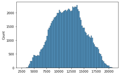
s_DE_emissions_tonnes = (df_fuels_DE
                         .multiply(1e3) # converting to MWh
                         [DE_fuel_to_co2_intensity.keys()]
                         .multiply(DE_fuel_to_co2_intensity.values())
                         .sum(axis=1)
                        )

s_DE_emissions_tonnes = s_DE_emissions_tonnes[s_DE_emissions_tonnes>2000]

sns.histplot(s_DE_emissions_tonnes)

<AxesSubplot:ylabel='Count'>

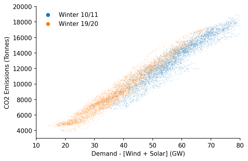
We'll do a quick plot of the change over time

df_DE = pd.DataFrame({
    'demand': df_fuels_DE.sum(axis=1),
    'dispatchable': df_fuels_DE.drop(columns=['Solar', 'Wind']).sum(axis=1),
    'emissions': s_DE_emissions_tonnes
}).dropna()

# Plotting
fig, ax = plt.subplots(dpi=150)

ax.scatter(df_DE.loc['2010-09':'2011-03', 'dispatchable'], df_DE.loc['2010-09':'2011-03', 'emissions'], s=0.1, alpha=0.25, label='Winter 10/11')
ax.scatter(df_DE.loc['2019-09':'2020-03', 'dispatchable'], df_DE.loc['2019-09':'2020-03', 'emissions'], s=0.1, alpha=0.25, label='Winter 19/20')

eda.hide_spines(ax)
ax.set_xlim(10, 80)
ax.set_ylim(3000, 20000)
ax.set_xlabel('Demand - [Wind + Solar] (GW)')
ax.set_ylabel('CO2 Emissions (Tonnes)')

lgnd = ax.legend(frameon=False) # Need to increase the legend marker size
lgnd.legendHandles[0]._sizes = [30]
lgnd.legendHandles[1]._sizes = [30]

for lh in lgnd.legendHandles: 
    lh.set_alpha(1)

Great Britain

We'll now do the same for the GB system

df_fuels_GB = pd.read_csv('../data/raw/electric_insights.csv')

df_fuels_GB = df_fuels_GB.set_index('local_datetime')
df_fuels_GB.index = pd.to_datetime(df_fuels_GB.index, utc=True).tz_convert('Europe/Berlin')

df_fuels_GB.head()

local_datetime	day_ahead_price	SP	imbalance_price	valueSum	temperature	TCO2_per_h	gCO2_per_kWh	nuclear	biomass	coal	...	demand	pumped_storage	wind_onshore	wind_offshore	belgian	dutch	french	ireland	northern_ireland	irish
2009-01-01 01:00:00+01:00	58.05	1	74.74	74.74	-0.6	21278	555	6.973	0	17.65	...	38.329	-0.404	nan	nan	0	0	1.977	0	0	-0.161
2009-01-01 01:30:00+01:00	56.33	2	74.89	74.89	-0.6	21442	558	6.968	0	17.77	...	38.461	-0.527	nan	nan	0	0	1.977	0	0	-0.16
2009-01-01 02:00:00+01:00	52.98	3	76.41	76.41	-0.6	21614	569	6.97	0	18.07	...	37.986	-1.018	nan	nan	0	0	1.977	0	0	-0.16
2009-01-01 02:30:00+01:00	50.39	4	37.73	37.73	-0.6	21320	578	6.969	0	18.022	...	36.864	-1.269	nan	nan	0	0	1.746	0	0	-0.16
2009-01-01 03:00:00+01:00	48.7	5	59	59	-0.6	21160	585	6.96	0	17.998	...	36.18	-1.566	nan	nan	0	0	1.73	0	0	-0.16

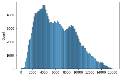
We'll source the carbon intensity data from DUKES where possible and Electric Insights where it isn't.

GB_fuel_to_co2_intensity = {
    'nuclear': 0, 
    'biomass': 0.121, # from EI 
    'coal': 0.921, # DUKES 2018 value
    'gas': 0.377, # DUKES 2018 value (lower than many CCGT estimates, let alone OCGT)
    'hydro': 0, 
    'pumped_storage': 0, 
    'solar': 0,
    'wind': 0,
    'belgian': 0.4,  
    'dutch': 0.474, # from EI 
    'french': 0.053, # from EI 
    'ireland': 0.458, # from EI 
    'northern_ireland': 0.458 # from EI 
}

s_GB_emissions_tonnes = (df_fuels_GB
                         .multiply(1e3*0.5) # converting to MWh
                         [GB_fuel_to_co2_intensity.keys()]
                         .multiply(GB_fuel_to_co2_intensity.values())
                         .sum(axis=1)
                        )

sns.histplot(s_GB_emissions_tonnes)

<AxesSubplot:ylabel='Count'>

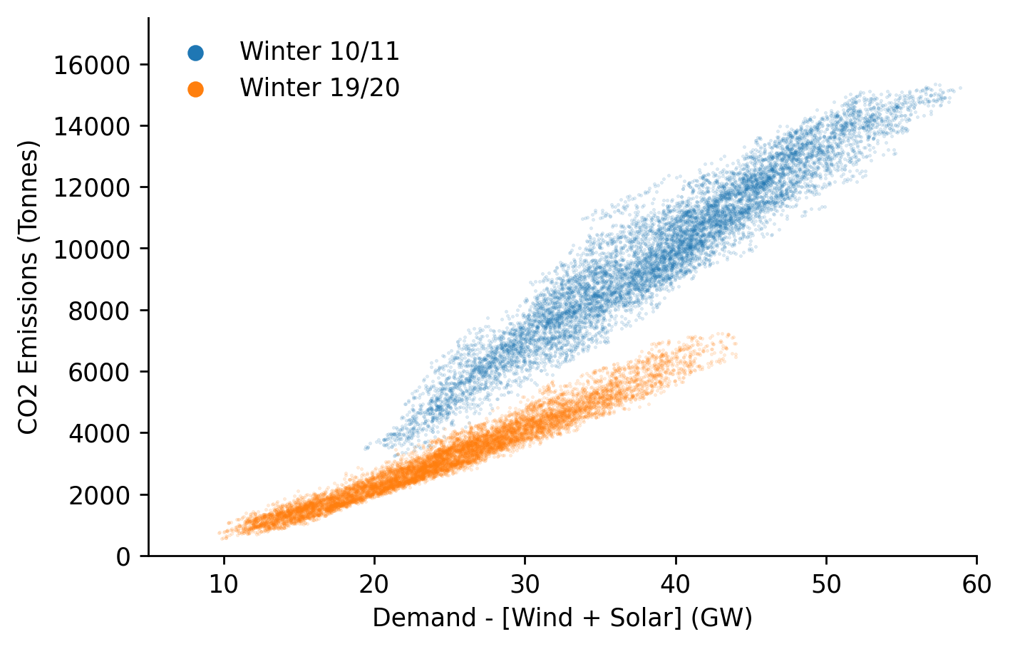
We'll do the same visualisation for GB of how the carbon intensity has changed over time.

Interestly we can see a clear fall in the carbon intensity of the GB dispatchable fleet, whereas with Germany the difference is negligible and if anything has slightly increased.

df_GB = pd.DataFrame({
    'demand': df_fuels_GB[GB_fuel_to_co2_intensity.keys()].sum(axis=1),
    'dispatchable': df_fuels_GB[GB_fuel_to_co2_intensity.keys()].drop(columns=['solar', 'wind']).sum(axis=1),
    'emissions': s_GB_emissions_tonnes
}).dropna()

# Plotting
fig, ax = plt.subplots(dpi=250)

ax.scatter(df_GB.loc['2010-09':'2011-03', 'dispatchable'], df_GB.loc['2010-09':'2011-03', 'emissions'], s=0.1, alpha=0.25, label='Winter 10/11')
ax.scatter(df_GB.loc['2019-09':'2020-03', 'dispatchable'], df_GB.loc['2019-09':'2020-03', 'emissions'], s=0.1, alpha=0.25, label='Winter 19/20')

eda.hide_spines(ax)
ax.set_xlim(5, 60)
ax.set_ylim(0, 17500)
ax.set_xlabel('Demand - [Wind + Solar] (GW)')
ax.set_ylabel('CO2 Emissions (Tonnes)')

lgnd = ax.legend(frameon=False) # Need to increase the legend marker size
lgnd.legendHandles[0]._sizes = [30]
lgnd.legendHandles[1]._sizes = [30]

for lh in lgnd.legendHandles: 
    lh.set_alpha(1)

Model Fitting

We're ready to define and fit our models

model_definitions = {
    'carbon_emissions_DE': {
        'dt_idx': df_DE.index,
        'x': df_DE['dispatchable'].values,
        'y': df_DE['emissions'].values,
        'reg_dates_start': '2010-01-04',
        'reg_dates_end': '2021-01-01',
        'reg_dates_freq': '13W',  
        'frac': 0.3, 
        'num_fits': 31, 
        'dates_smoothing_value': 26, 
        'dates_smoothing_units': 'W',
        'fit_kwarg_sets': surface.get_fit_kwarg_sets(qs=[0.16, 0.5, 0.84])
    },
    'carbon_emissions_GB': {
        'dt_idx': df_GB.index,
        'x': df_GB['dispatchable'].values,
        'y': df_GB['emissions'].values,
        'reg_dates_start': '2010-01-04',
        'reg_dates_end': '2021-01-01',
        'reg_dates_freq': '13W',  
        'frac': 0.3, 
        'num_fits': 31, 
        'dates_smoothing_value': 26,
        'dates_smoothing_units': 'W',
        'fit_kwarg_sets': surface.get_fit_kwarg_sets(qs=[0.16, 0.5, 0.84])
    }
}

surface.fit_models(model_definitions, models_dir)

carbon_emissions_DE 100% 4/4 [00:00<00:00, 0.00s/it]

carbon_emissions_GB 100% 4/4 [00:00<00:00, 0.00s/it]

German Model Evaluation & Carbon Savings Calculations

We'll start by loading in the model

%%time

DE_model_fp = '../data/models/carbon_emissions_DE_p50.pkl'
DE_smooth_dates = pickle.load(open(DE_model_fp, 'rb'))

DE_x_pred = np.linspace(-5, 91, 961)
DE_dt_pred = pd.date_range('2010-01-01', '2020-12-31', freq='D')

df_DE_pred = DE_smooth_dates.predict(x_pred=DE_x_pred, dt_pred=DE_dt_pred)
df_DE_pred.index = np.round(df_DE_pred.index, 1)

df_DE_pred.head()

Wall time: 3.22 s

Unnamed: 0	2010-01-01	2010-01-02	2010-01-03	2010-01-04	2010-01-05	2010-01-06	2010-01-07	2010-01-08	2010-01-09	2010-01-10	...	2020-12-22	2020-12-23	2020-12-24	2020-12-25	2020-12-26	2020-12-27	2020-12-28	2020-12-29	2020-12-30	2020-12-31
-5	3886.65	3879.82	3873.02	3866.24	3859.49	3852.78	3846.09	3839.43	3832.81	3826.22	...	90.9967	89.6073	88.2112	86.8081	85.3975	83.9787	82.5515	81.1158	79.6717	78.2193
-4.9	3892.08	3885.26	3878.48	3871.72	3864.99	3858.3	3851.63	3844.99	3838.39	3831.82	...	109.687	108.304	106.915	105.518	104.113	102.701	101.28	99.8512	98.4136	96.9678
-4.8	3897.58	3890.78	3884.01	3877.28	3870.57	3863.89	3857.24	3850.62	3844.04	3837.48	...	128.39	127.013	125.63	124.24	122.842	121.436	120.021	118.599	117.168	115.728
-4.7	3903.14	3896.36	3889.62	3882.89	3876.2	3869.54	3862.91	3856.31	3849.75	3843.21	...	147.105	145.734	144.357	142.973	141.581	140.182	138.774	137.358	135.933	134.501
-4.6	3908.73	3901.97	3895.24	3888.54	3881.86	3875.22	3868.61	3862.03	3855.48	3848.96	...	165.828	164.463	163.092	161.715	160.33	158.936	157.535	156.125	154.707	153.281

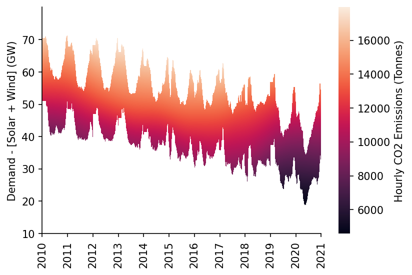
We'll then visualise the surface prediction as a heatmap

df_DE_dispatchable_lims = moe.construct_dispatchable_lims_df(df_DE['dispatchable'], rolling_w=6)
df_DE_pred_mask = moe.construct_pred_mask_df(df_DE_pred, df_DE_dispatchable_lims)

# Plotting
min_y = 10
max_y = 80
fig, ax = plt.subplots(dpi=150)

htmp = sns.heatmap(df_DE_pred[min_y:max_y].where(df_DE_pred_mask[min_y:max_y], np.nan).iloc[::-1], ax=ax, cbar_kws={'label': 'Hourly CO2 Emissions (Tonnes)'})

moe.set_ticks(ax, np.arange(min_y, max_y, 10), axis='y')
moe.set_date_ticks(ax, '2010-01-01', '2021-01-01', freq='1YS', date_format='%Y', axis='x')

for _, spine in htmp.spines.items():
    spine.set_visible(True)
eda.hide_spines(ax)

ax.set_ylabel('Demand - [Solar + Wind] (GW)')

C:\Users\Ayrto\anaconda3\envs\MOE\lib\site-packages\sklearn\utils\validation.py:63: FutureWarning: Arrays of bytes/strings is being converted to decimal numbers if dtype='numeric'. This behavior is deprecated in 0.24 and will be removed in 1.1 (renaming of 0.26). Please convert your data to numeric values explicitly instead.
  return f(*args, **kwargs)





Text(69.58333333333334, 0.5, 'Demand - [Solar + Wind] (GW)')

We'll calculate the model metrics

s_DE_pred_ts_dispatch, s_DE_pred_ts_demand = moe.get_model_pred_ts(df_DE['dispatchable'], DE_model_fp, s_demand=df_DE['demand'], x_pred=DE_x_pred, dt_pred=DE_dt_pred)
s_DE_err = s_DE_pred_ts_dispatch - df_DE.loc[s_DE_pred_ts_dispatch.index, 'emissions']
metrics = moe.calc_error_metrics(s_DE_err)

metrics

C:\Users\Ayrto\anaconda3\envs\MOE\lib\site-packages\pandas\core\indexes\base.py:5277: FutureWarning: Indexing a timezone-aware DatetimeIndex with a timezone-naive datetime is deprecated and will raise KeyError in a future version.  Use a timezone-aware object instead.
  start_slice, end_slice = self.slice_locs(start, end, step=step, kind=kind)

100% 48050/96191 [01:28<00:00, 0.00s/it]

100% 0/96191 [01:20<00:00, 0.00s/it]

{'median_abs_err': 603.7669189236494,
 'mean_abs_err': 750.7665511092414,
 'root_mean_square_error': 967.8069705064318}

And \(r^{2}\) score

r2_score(df_DE.loc[s_DE_pred_ts_dispatch.index, 'emissions'], s_DE_pred_ts_dispatch)

0.9139682818721121

We're now ready to calculate the total savings

start_date = '2010'
end_date = '2020'

s_DE_MOE = s_DE_pred_ts_demand - s_DE_pred_ts_dispatch
s_DE_MOE = s_DE_MOE.dropna()

total_saving = s_DE_MOE[start_date:end_date].sum()

print(f"The total saving between {start_date} and {end_date} was {total_saving:,.0f} Tonnes")

The total saving between 2010 and 2020 was 318,923,308 Tonnes

And get some context for the average and total emissions over the same period

s_DE_emissions = df_DE['emissions'].loc[s_DE_MOE.index]

avg_DE_HH_emissions = s_DE_emissions.mean()
total_DE_emissions = s_DE_emissions[start_date:end_date].sum()

avg_DE_HH_emissions, total_DE_emissions

(11870.320551662837, 1141818004.185)

We'll calculate the average percentage emissions reduction due to the MOE

total_saving/(total_DE_emissions+total_saving)

0.21832976535024085

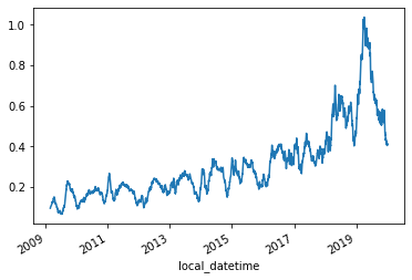
Finally we'll generate the MOE percentage time-series

s_DE_emissions_rolling = s_DE_emissions.rolling(48*28).mean().dropna()
s_DE_MOE_rolling = s_DE_MOE.rolling(48*28).mean().dropna()

s_DE_MOE_pct_reduction = s_DE_MOE_rolling/s_DE_emissions_rolling

s_DE_MOE_pct_reduction.plot()

<AxesSubplot:xlabel='local_datetime'>

British Model Evaluation & Carbon Savings Calculations

We'll start by loading in the model

%%time

start_date = '2010-01-01'
end_date = '2020-12-31'

GB_model_fp = '../data/models/carbon_emissions_GB_p50.pkl'
GB_smooth_dates = pickle.load(open(GB_model_fp, 'rb'))

GB_x_pred = np.linspace(-5, 91, 961)
GB_dt_pred = pd.date_range(start_date, end_date, freq='D')

df_GB_pred = GB_smooth_dates.predict(x_pred=GB_x_pred, dt_pred=GB_dt_pred)
df_GB_pred.index = np.round(df_GB_pred.index, 1)

df_GB_pred.head()

Wall time: 3.73 s

Unnamed: 0	2010-01-01	2010-01-02	2010-01-03	2010-01-04	2010-01-05	2010-01-06	2010-01-07	2010-01-08	2010-01-09	2010-01-10	...	2020-12-22	2020-12-23	2020-12-24	2020-12-25	2020-12-26	2020-12-27	2020-12-28	2020-12-29	2020-12-30	2020-12-31
-5	-3464.32	-3464.5	-3464.68	-3464.85	-3465.03	-3465.2	-3465.38	-3465.55	-3465.72	-3465.89	...	-1132.67	-1132.65	-1132.62	-1132.59	-1132.57	-1132.54	-1132.52	-1132.49	-1132.46	-1132.44
-4.9	-3440	-3440.17	-3440.33	-3440.49	-3440.66	-3440.82	-3440.98	-3441.14	-3441.29	-3441.45	...	-1119.73	-1119.7	-1119.67	-1119.65	-1119.62	-1119.6	-1119.57	-1119.55	-1119.52	-1119.49
-4.8	-3415.64	-3415.79	-3415.94	-3416.1	-3416.24	-3416.39	-3416.54	-3416.68	-3416.83	-3416.97	...	-1106.78	-1106.75	-1106.73	-1106.7	-1106.68	-1106.65	-1106.63	-1106.6	-1106.57	-1106.55
-4.7	-3391.24	-3391.38	-3391.52	-3391.66	-3391.79	-3391.93	-3392.06	-3392.2	-3392.33	-3392.46	...	-1093.84	-1093.81	-1093.78	-1093.76	-1093.73	-1093.71	-1093.68	-1093.66	-1093.63	-1093.6
-4.6	-3366.81	-3366.93	-3367.06	-3367.18	-3367.31	-3367.43	-3367.55	-3367.67	-3367.79	-3367.91	...	-1080.89	-1080.87	-1080.84	-1080.82	-1080.79	-1080.77	-1080.74	-1080.71	-1080.69	-1080.66

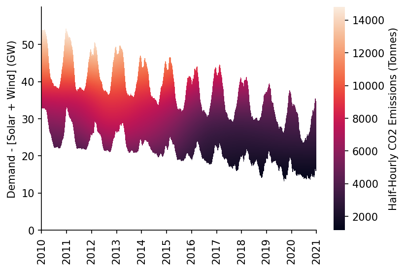
We'll then visualise the surface prediction as a heatmap

df_GB_dispatchable_lims = moe.construct_dispatchable_lims_df(df_GB.loc[start_date:end_date, 'dispatchable'], rolling_w=6)
df_GB_pred_mask = moe.construct_pred_mask_df(df_GB_pred, df_GB_dispatchable_lims)

# Plotting
min_y = 0
max_y = 60
fig, ax = plt.subplots(dpi=150)

htmp = sns.heatmap(df_GB_pred[min_y:max_y].where(df_GB_pred_mask[min_y:max_y], np.nan).iloc[::-1], ax=ax, cbar_kws={'label': 'Half-Hourly CO2 Emissions (Tonnes)'})

moe.set_ticks(ax, np.arange(min_y, max_y, 10), axis='y')
moe.set_date_ticks(ax, '2010-01-01', '2021-01-01', freq='1YS', date_format='%Y', axis='x')

for _, spine in htmp.spines.items():
    spine.set_visible(True)
eda.hide_spines(ax)

ax.set_ylabel('Demand - [Solar + Wind] (GW)')

C:\Users\Ayrto\anaconda3\envs\MOE\lib\site-packages\sklearn\utils\validation.py:63: FutureWarning: Arrays of bytes/strings is being converted to decimal numbers if dtype='numeric'. This behavior is deprecated in 0.24 and will be removed in 1.1 (renaming of 0.26). Please convert your data to numeric values explicitly instead.
  return f(*args, **kwargs)





Text(69.58333333333334, 0.5, 'Demand - [Solar + Wind] (GW)')

We'll calculate the model metrics

s_GB_pred_ts_dispatch, s_GB_pred_ts_demand = moe.get_model_pred_ts(df_GB['dispatchable'], GB_model_fp, s_demand=df_GB['demand'], x_pred=GB_x_pred, dt_pred=GB_dt_pred)
s_GB_err = s_GB_pred_ts_dispatch - df_GB.loc[s_GB_pred_ts_dispatch.index, 'emissions']
metrics = moe.calc_error_metrics(s_GB_err)

metrics

C:\Users\Ayrto\anaconda3\envs\MOE\lib\site-packages\pandas\core\indexes\base.py:5277: FutureWarning: Indexing a timezone-aware DatetimeIndex with a timezone-naive datetime is deprecated and will raise KeyError in a future version.  Use a timezone-aware object instead.
  start_slice, end_slice = self.slice_locs(start, end, step=step, kind=kind)

100% 130764/192336 [02:32<00:00, 0.00s/it]

100% 0/192336 [02:11<00:00, 0.00s/it]

{'median_abs_err': 330.24369388573996,
 'mean_abs_err': 476.21722650533655,
 'root_mean_square_error': 661.7182203091455}

And \(r^{2}\) score

r2_score(df_GB.loc[s_GB_pred_ts_dispatch.index, 'emissions'], s_GB_pred_ts_dispatch)

0.9557674211115541

We're now ready to calculate the total savings

s_GB_MOE = s_GB_pred_ts_demand - s_GB_pred_ts_dispatch
s_GB_MOE = s_GB_MOE.dropna()

total_saving = s_GB_MOE[start_date:end_date].sum()

print(f"The total saving between {start_date} and {end_date} was {total_saving:,.0f} Tonnes")

The total saving between 2010-01-01 and 2020-12-31 was 221,069,470 Tonnes

And get some context for the average and total emissions over the same period

s_GB_emissions = df_GB['emissions'].loc[s_GB_MOE.index]

avg_GB_HH_emissions = s_GB_emissions.mean()
total_GB_emissions = s_GB_emissions[start_date:end_date].sum()

avg_GB_HH_emissions, total_GB_emissions

(6034.469929827791, 1160645808.423358)

We'll calculate the average percentage emissions reduction due to the MOE

total_saving/(total_GB_emissions+total_saving)

0.15999639957299291

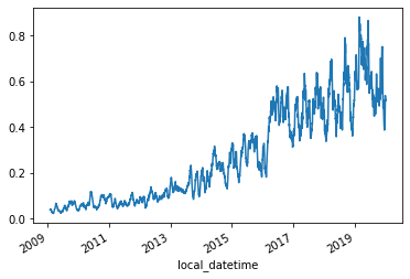
Finally we'll generate the MOE percentage time-series

s_GB_emissions_rolling = s_GB_emissions.rolling(48*28).mean().dropna()
s_GB_MOE_rolling = s_GB_MOE.rolling(48*28).mean().dropna()

s_GB_MOE_pct_reduction = s_GB_MOE_rolling/s_GB_emissions_rolling

s_GB_MOE_pct_reduction.plot()

<AxesSubplot:xlabel='local_datetime'>

Plots

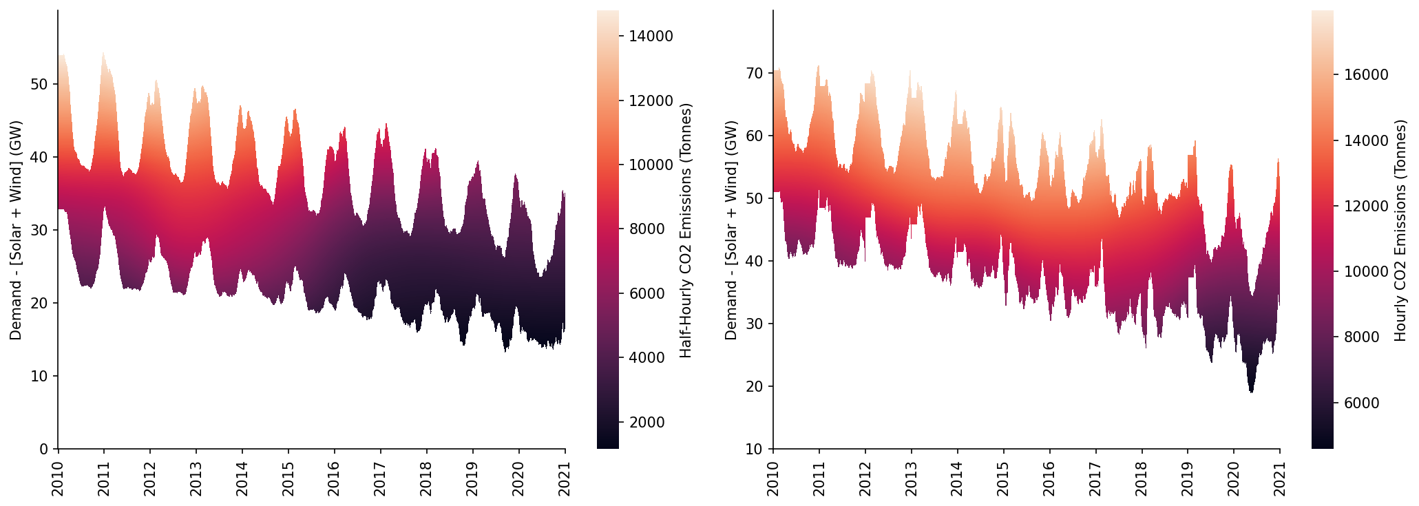
In this section we'll generate some of the plots needed for the paper, starting with the heatmap of the emissions surfaces

fig, axs = plt.subplots(dpi=150, ncols=2, figsize=(14, 5))

# GB
ax = axs[0]
min_y = 0
max_y = 60

htmp = sns.heatmap(df_GB_pred[min_y:max_y].where(df_GB_pred_mask[min_y:max_y], np.nan).iloc[::-1], ax=ax, cbar_kws={'label': 'Half-Hourly CO2 Emissions (Tonnes)'})

moe.set_ticks(ax, np.arange(min_y, max_y, 10), axis='y')
moe.set_date_ticks(ax, '2010-01-01', '2021-01-01', freq='1YS', date_format='%Y', axis='x')

for _, spine in htmp.spines.items():
    spine.set_visible(True)
eda.hide_spines(ax)

ax.set_ylabel('Demand - [Solar + Wind] (GW)')

# DE
ax = axs[1]
min_y = 10
max_y = 80

htmp = sns.heatmap(df_DE_pred[min_y:max_y].where(df_DE_pred_mask[min_y:max_y], np.nan).iloc[::-1], ax=ax, cbar_kws={'label': 'Hourly CO2 Emissions (Tonnes)'})

moe.set_ticks(ax, np.arange(min_y, max_y, 10), axis='y')
moe.set_date_ticks(ax, '2010-01-01', '2021-01-01', freq='1YS', date_format='%Y', axis='x')

for _, spine in htmp.spines.items():
    spine.set_visible(True)
eda.hide_spines(ax)

ax.set_ylabel('Demand - [Solar + Wind] (GW)')

fig.tight_layout()

C:\Users\Ayrto\anaconda3\envs\MOE\lib\site-packages\sklearn\utils\validation.py:63: FutureWarning: Arrays of bytes/strings is being converted to decimal numbers if dtype='numeric'. This behavior is deprecated in 0.24 and will be removed in 1.1 (renaming of 0.26). Please convert your data to numeric values explicitly instead.
  return f(*args, **kwargs)
C:\Users\Ayrto\anaconda3\envs\MOE\lib\site-packages\sklearn\utils\validation.py:63: FutureWarning: Arrays of bytes/strings is being converted to decimal numbers if dtype='numeric'. This behavior is deprecated in 0.24 and will be removed in 1.1 (renaming of 0.26). Please convert your data to numeric values explicitly instead.
  return f(*args, **kwargs)

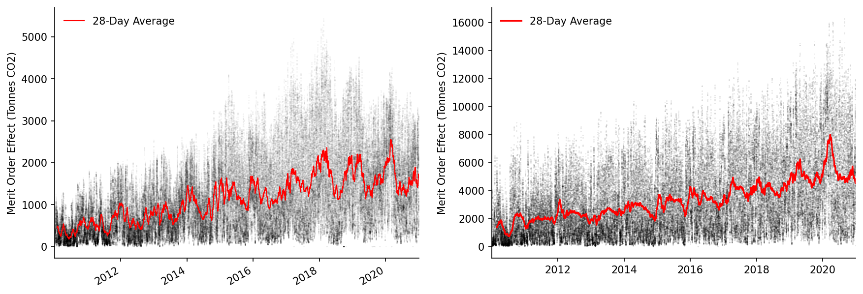
We'll also plot the MOE time-series

fig, axs = plt.subplots(dpi=150, ncols=2, figsize=(14, 5))

# GB
ax = axs[0]

ax.scatter(s_GB_MOE.index, s_GB_MOE, s=0.01, alpha=0.2, color='k', label=None)
s_GB_MOE_rolling.plot(color='r', linewidth=1, ax=ax, label='28-Day Average')

eda.hide_spines(ax)
# ax.set_ylim(0, 40)
ax.set_xlim(pd.to_datetime('2010'), pd.to_datetime('2021'))
ax.set_xlabel('')
ax.set_ylabel('Merit Order Effect (Tonnes CO2)')
ax.legend(frameon=False)

# DE
ax = axs[1]

ax.scatter(s_DE_MOE.index, s_DE_MOE, s=0.05, alpha=0.2, color='k', label=None)
ax.plot(s_DE_MOE_rolling.index, s_DE_MOE_rolling, color='r', linewidth=1.5, label='28-Day Average')

eda.hide_spines(ax)
ax.set_xlim(pd.to_datetime('2010'), pd.to_datetime('2021'))
ax.set_xlabel('')
ax.set_ylabel('Merit Order Effect (Tonnes CO2)')
ax.legend(frameon=False)

<matplotlib.legend.Legend at 0x181ff7c1af0>

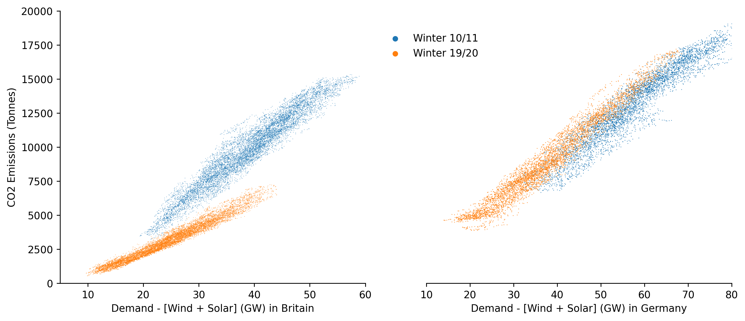
Finally we'll visualise the changing emissions from dispatchable generation between the two countries

fig, axs = plt.subplots(dpi=250, ncols=2, figsize=(12, 5))

# GB
ax = axs[0]
ax.scatter(df_GB.loc['2010-09':'2011-03', 'dispatchable'], df_GB.loc['2010-09':'2011-03', 'emissions'], s=0.25, linewidth=0, alpha=1, label='Winter 10/11')
ax.scatter(df_GB.loc['2019-09':'2020-03', 'dispatchable'], df_GB.loc['2019-09':'2020-03', 'emissions'], s=0.25, linewidth=0, alpha=1, label='Winter 19/20')

eda.hide_spines(ax)
ax.set_xlim(5, 60)
ax.set_xlabel('Demand - [Wind + Solar] (GW) in Britain')
ax.set_ylabel('CO2 Emissions (Tonnes)')

# DE
ax = axs[1]
ax.scatter(df_DE.loc['2010-09':'2011-03', 'dispatchable'], df_DE.loc['2010-09':'2011-03', 'emissions'], s=0.5, linewidth=0, alpha=1, label='Winter 10/11')
ax.scatter(df_DE.loc['2019-09':'2020-03', 'dispatchable'], df_DE.loc['2019-09':'2020-03', 'emissions'], s=0.5, linewidth=0, alpha=1, label='Winter 19/20')

eda.hide_spines(ax, positions=['top', 'left', 'right'])
ax.set_yticks([])
ax.set_xlim(10, 80)
ax.set_xlabel('Demand - [Wind + Solar] (GW) in Germany')

lgnd = ax.legend(frameon=False, bbox_to_anchor=(0.2, 0.95)) 
lgnd.legendHandles[0]._sizes = [30]
lgnd.legendHandles[1]._sizes = [30]

for lh in lgnd.legendHandles: 
    lh.set_alpha(1)

for ax in axs:
    ax.set_ylim(0, 20000)

Saving Results

Additionaly we'll save the time-series predictions and model metrics, starting with the GB time-series

df_GB_results_ts = pd.DataFrame({
    'prediction': s_GB_pred_ts_dispatch,
    'counterfactual': s_GB_pred_ts_demand,
    'observed': df_GB.loc[s_GB_pred_ts_dispatch.index, 'emissions'],
    'moe': s_GB_MOE
})

df_GB_results_ts.head()

local_datetime	prediction	counterfactual	observed	moe
2010-01-01 01:00:00+01:00	8414.72	8861.95	7949.28	447.23
2010-01-01 01:30:00+01:00	8535.22	8986.13	8030.29	450.914
2010-01-01 02:00:00+01:00	8414.72	8820.73	7974.91	406.012
2010-01-01 02:30:00+01:00	7983.82	8454.75	7707.51	470.937
2010-01-01 03:00:00+01:00	7645.47	8060.81	7456.2	415.345

Which we'll save to csv

df_GB_results_ts.to_csv('../data/results/GB_carbon.csv')

Then the DE time-series

df_DE_results_ts = pd.DataFrame({
    'prediction': s_DE_pred_ts_dispatch,
    'counterfactual': s_DE_pred_ts_demand,
    'observed': df_DE.loc[s_DE_pred_ts_dispatch.index, 'emissions'],
    'moe': s_DE_MOE
})

df_DE_results_ts.to_csv('../data/results/DE_carbon.csv')

df_DE_results_ts.head()

local_datetime	prediction	counterfactual	observed	moe
2010-01-04 00:00:00+01:00	11981.6	12179	11883.8	197.359
2010-01-04 01:00:00+01:00	11518.7	11694.3	11488.6	175.594
2010-01-04 02:00:00+01:00	11400.5	11577.4	11228.5	176.903
2010-01-04 03:00:00+01:00	11071.5	11251.9	10962.7	180.385
2010-01-04 04:00:00+01:00	11311.5	11518.7	10892.5	207.187