Estimation of Price Surfaces
![]()
This notebook outlines how to specify different variants the model, then proceeds to fit them.
Imports
#exports
import pandas as pd
import numpy as np

import os
import pickle
from tqdm import tqdm

from moepy import lowess, eda
import seaborn as sns
import matplotlib.pyplot as plt
User Inputs
models_dir = '../data/models'
load_existing_model = True
Loading & Cleaning Data
We'll start by loading in ...
%%time

df_EI = eda.load_EI_df('../data/raw/electric_insights.csv')

df_EI.head()
Wall time: 1.69 s
| local_datetime | day_ahead_price | SP | imbalance_price | valueSum | temperature | TCO2_per_h | gCO2_per_kWh | nuclear | biomass | coal | ... | demand | pumped_storage | wind_onshore | wind_offshore | belgian | dutch | french | ireland | northern_ireland | irish |
|---|---|---|---|---|---|---|---|---|---|---|---|---|---|---|---|---|---|---|---|---|---|
| 2009-01-01 00:00:00+00:00 | 58.05 | 1 | 74.74 | 74.74 | -0.6 | 21278 | 555 | 6.973 | 0 | 17.65 | ... | 38.329 | -0.404 | nan | nan | 0 | 0 | 1.977 | 0 | 0 | -0.161 |
| 2009-01-01 00:30:00+00:00 | 56.33 | 2 | 74.89 | 74.89 | -0.6 | 21442 | 558 | 6.968 | 0 | 17.77 | ... | 38.461 | -0.527 | nan | nan | 0 | 0 | 1.977 | 0 | 0 | -0.16 |
| 2009-01-01 01:00:00+00:00 | 52.98 | 3 | 76.41 | 76.41 | -0.6 | 21614 | 569 | 6.97 | 0 | 18.07 | ... | 37.986 | -1.018 | nan | nan | 0 | 0 | 1.977 | 0 | 0 | -0.16 |
| 2009-01-01 01:30:00+00:00 | 50.39 | 4 | 37.73 | 37.73 | -0.6 | 21320 | 578 | 6.969 | 0 | 18.022 | ... | 36.864 | -1.269 | nan | nan | 0 | 0 | 1.746 | 0 | 0 | -0.16 |
| 2009-01-01 02:00:00+00:00 | 48.7 | 5 | 59 | 59 | -0.6 | 21160 | 585 | 6.96 | 0 | 17.998 | ... | 36.18 | -1.566 | nan | nan | 0 | 0 | 1.73 | 0 | 0 | -0.16 |
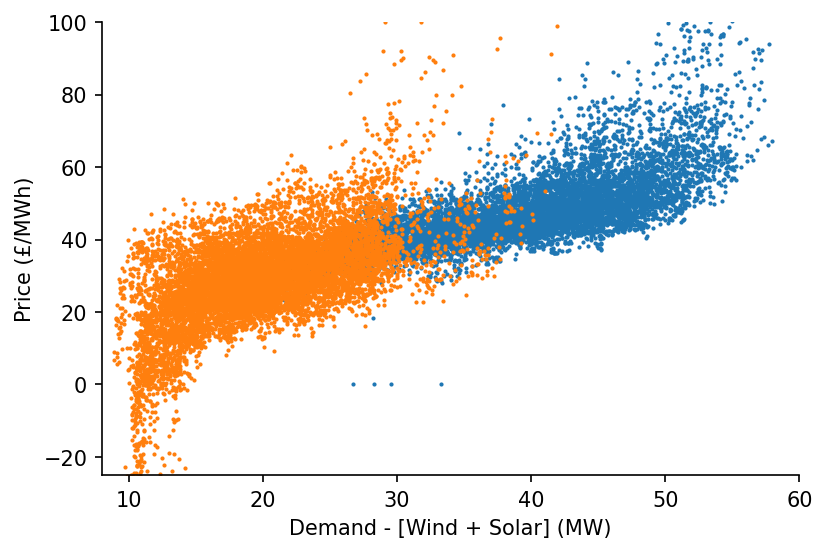
... and cleaning the GB data
df_EI_model = df_EI[['day_ahead_price', 'demand', 'solar', 'wind']].dropna()

s_demand = df_EI_model['demand']
s_price = df_EI_model['day_ahead_price']
s_dispatchable = df_EI_model['demand'] - df_EI_model[['solar', 'wind']].sum(axis=1)

# Plotting
fig, ax = plt.subplots(dpi=150)

ax.scatter(s_dispatchable['2010-09':'2011-03'], s_price['2010-09':'2011-03'], s=1)
ax.scatter(s_dispatchable['2020-03':'2020-09'], s_price['2020-03':'2020-09'], s=1)

eda.hide_spines(ax)
ax.set_xlim(8, 60)
ax.set_ylim(-25, 100)
ax.set_xlabel('Demand - [Wind + Solar] (MW)')
ax.set_ylabel('Price (£/MWh)')
Text(0, 0.5, 'Price (£/MWh)')
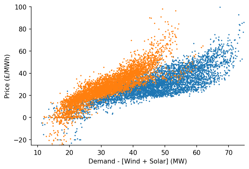
As well as the DE data
df_DE = eda.load_DE_df('../data/raw/energy_charts.csv', '../data/raw/ENTSOE_DE_price.csv')

df_DE_model = df_DE[['price', 'demand', 'Solar', 'Wind']].dropna()

s_DE_demand = df_DE_model['demand']
s_DE_price = df_DE_model['price']
s_DE_dispatchable = df_DE_model['demand'] - df_DE_model[['Solar', 'Wind']].sum(axis=1)

# Plotting
fig, ax = plt.subplots(dpi=150)

ax.scatter(s_DE_dispatchable['2015-09':'2016-03'], s_DE_price['2015-09':'2016-03'], s=1)
ax.scatter(s_DE_dispatchable['2020-03':'2020-09'], s_DE_price['2020-03':'2020-09'], s=1)

eda.hide_spines(ax)
ax.set_xlim(8, 75)
ax.set_ylim(-25, 100)
ax.set_xlabel('Demand - [Wind + Solar] (MW)')
ax.set_ylabel('Price (£/MWh)')
Text(0, 0.5, 'Price (£/MWh)')
Results Wrapper
We'll start defining each of the price models that we'll fit, using the PicklableFunction class to ensure that all of our models can be saved for later use.
#exports
import copy
import types
import marshal

class PicklableFunction:
    """Provides a wrapper to ensure functions can be pickled"""
    def __init__(self, fun):
        self._fun = fun

    def __call__(self, *args, **kwargs):
        return self._fun(*args, **kwargs)

    def __getstate__(self):
        try:
            return pickle.dumps(self._fun)
        except Exception:
            return marshal.dumps((self._fun.__code__, self._fun.__name__))

    def __setstate__(self, state):
        try:
            self._fun = pickle.loads(state)
        except Exception:
            code, name = marshal.loads(state)
            self._fun = types.FunctionType(code, {}, name)

        return

def get_fit_kwarg_sets(qs=np.linspace(0.1, 0.9, 9)):
    """Helper to generate kwargs for the `fit` method of `Lowess`"""
    fit_kwarg_sets = [
        # quantile lowess
        {
            'name': f'p{int(q*100)}',
            'lowess_kwargs': {'reg_func': PicklableFunction(lowess.calc_quant_reg_betas)},
            'q': q,
        }
        for q in qs

        # standard lowess
    ] + [{'name': 'average'}]

    return fit_kwarg_sets
model_definitions = {
    'DAM_price_GB': {
        'dt_idx': s_dispatchable.index,
        'x': s_dispatchable.values,
        'y': s_price.values,
        'reg_dates_start': '2009-01-01',
        'reg_dates_end': '2021-01-01',
        'reg_dates_freq': '13W', # 13
        'frac': 0.3,
        'num_fits': 31, # 31
        'dates_smoothing_value': 26, # 26
        'dates_smoothing_units': 'W',
        'fit_kwarg_sets': get_fit_kwarg_sets(qs=[0.16, 0.5, 0.84])
    },
    'DAM_price_demand_GB': {
        'dt_idx': s_demand.index,
        'x': s_demand.values,
        'y': s_price.values,
        'reg_dates_start': '2009-01-01',
        'reg_dates_end': '2021-01-01',
        'reg_dates_freq': '13W', # 13
        'frac': 0.3,
        'num_fits': 31, # 31
        'dates_smoothing_value': 26, # 26
        'dates_smoothing_units': 'W',
        'fit_kwarg_sets': get_fit_kwarg_sets(qs=[0.5])
    },
    'DAM_price_DE': {
        'dt_idx': s_DE_dispatchable.index,
        'x': s_DE_dispatchable.values,
        'y': s_DE_price.values,
        'reg_dates_start': '2015-01-04',
        'reg_dates_end': '2021-01-01',
        'reg_dates_freq': '13W', # 13
        'frac': 0.3,
        'num_fits': 31, # 31
        'dates_smoothing_value': 26, # 26
        'dates_smoothing_units': 'W',
        'fit_kwarg_sets': get_fit_kwarg_sets(qs=[0.16, 0.5, 0.84])
    },
    'DAM_price_demand_DE': {
        'dt_idx': s_DE_dispatchable.index,
        'x': s_DE_demand.values,
        'y': s_DE_price.values,
        'reg_dates_start': '2015-01-04',
        'reg_dates_end': '2021-01-01',
        'reg_dates_freq': '13W', # 13
        'frac': 0.3,
        'num_fits': 31, # 31
        'dates_smoothing_value': 26, # 26
        'dates_smoothing_units': 'W',
        'fit_kwarg_sets': get_fit_kwarg_sets(qs=[0.5])
    }
}
We'll now take these model definitions to fit and save them
#exports
def fit_models(model_definitions, models_dir):
    """Fits LOWESS variants using the specified model definitions"""
    for model_parent_name, model_spec in model_definitions.items():
        for fit_kwarg_set in tqdm(model_spec['fit_kwarg_sets'], desc=model_parent_name):
            run_name = fit_kwarg_set.pop('name')
            model_name = f'{model_parent_name}_{run_name}'

            if f'{model_name}.pkl' not in os.listdir(models_dir):
                smooth_dates = lowess.SmoothDates()

                reg_dates = pd.date_range(
                    model_spec['reg_dates_start'],
                    model_spec['reg_dates_end'],
                    freq=model_spec['reg_dates_freq']
                )

                smooth_dates.fit(
                    model_spec['x'],
                    model_spec['y'],
                    dt_idx=model_spec['dt_idx'],
                    reg_dates=reg_dates,
                    frac=model_spec['frac'],
                    threshold_value=model_spec['dates_smoothing_value'],
                    threshold_units=model_spec['dates_smoothing_units'],
                    num_fits=model_spec['num_fits'],
                    **fit_kwarg_set
                )

                model_fp = f'{models_dir}/{model_name}.pkl'
                pickle.dump(smooth_dates, open(model_fp, 'wb'))

                del smooth_dates
fit_models(model_definitions, models_dir)
100%
4/4
[00:00<00:00, 0.00s/it]
100%
2/2
[00:00<00:00, 0.00s/it]
100%
4/4
[00:00<00:00, 0.00s/it]
100%
2/2
[00:00<00:00, 0.00s/it]
We'll load one of the models in
%%time

if load_existing_model == True:
    smooth_dates = pickle.load(open(f'{models_dir}/DAM_price_GB_p50.pkl', 'rb'))
else:
    lowess_kwargs = {}
    reg_dates = pd.date_range('2009-01-01', '2021-01-01', freq='13W')

    smooth_dates = lowess.SmoothDates()
    smooth_dates.fit(s_dispatchable.values, s_price.values, dt_idx=s_dispatchable.index,
                     reg_dates=reg_dates, frac=0.3, num_fits=31, threshold_value=26, lowess_kwargs=lowess_kwargs)
Wall time: 2.7 s
And create a prediction surface using it
%%time

x_pred = np.linspace(8, 60, 521)
dt_pred = pd.date_range('2009-01-01', '2021-01-01', freq='1W')

df_pred = smooth_dates.predict(x_pred=x_pred, dt_pred=dt_pred)

df_pred.head()
Wall time: 346 ms
| Unnamed: 0 | 2009-01-04 | 2009-01-11 | 2009-01-18 | 2009-01-25 | 2009-02-01 | 2009-02-08 | 2009-02-15 | 2009-02-22 | 2009-03-01 | 2009-03-08 | ... | 2020-10-25 | 2020-11-01 | 2020-11-08 | 2020-11-15 | 2020-11-22 | 2020-11-29 | 2020-12-06 | 2020-12-13 | 2020-12-20 | 2020-12-27 |
|---|---|---|---|---|---|---|---|---|---|---|---|---|---|---|---|---|---|---|---|---|---|
| 8 | -7.66001 | -7.78927 | -7.91081 | -8.02572 | -8.13481 | -8.23875 | -8.33813 | -8.43345 | -8.52519 | -8.61382 | ... | 10.2354 | 10.292 | 10.3476 | 10.4021 | 10.4557 | 10.5085 | 10.5611 | 10.6143 | 10.6691 | 10.7271 |
| 8.1 | -7.46772 | -7.59637 | -7.71734 | -7.83171 | -7.94028 | -8.04374 | -8.14266 | -8.23754 | -8.32887 | -8.41709 | ... | 10.4429 | 10.4994 | 10.5548 | 10.6092 | 10.6627 | 10.7154 | 10.7679 | 10.821 | 10.8758 | 10.9336 |
| 8.2 | -7.27561 | -7.40364 | -7.52404 | -7.63785 | -7.74592 | -7.84889 | -7.94734 | -8.04178 | -8.13268 | -8.22049 | ... | 10.6503 | 10.7066 | 10.7619 | 10.8162 | 10.8695 | 10.9222 | 10.9746 | 11.0276 | 11.0823 | 11.1401 |
| 8.3 | -7.08366 | -7.21108 | -7.33089 | -7.44416 | -7.5517 | -7.65418 | -7.75217 | -7.84616 | -7.93663 | -8.02403 | ... | 10.8576 | 10.9138 | 10.9689 | 11.023 | 11.0763 | 11.1288 | 11.1812 | 11.2341 | 11.2888 | 11.3464 |
| 8.4 | -6.89188 | -7.01867 | -7.13789 | -7.25061 | -7.35763 | -7.45962 | -7.55713 | -7.65067 | -7.74071 | -7.82769 | ... | 11.0648 | 11.1208 | 11.1757 | 11.2298 | 11.2829 | 11.3353 | 11.3876 | 11.4405 | 11.4951 | 11.5527 |