.ipynb .pdf

open issue

Binder Live Code

Contents

Spatial Interpolation - Part 1

Analysis Preparation

Imports

All of these libraries should have been previously installed during the environment set-up, if they have not been installed already you can use install.packages(c("raster", "rgdal", "ape", "scales", "deldir", "gstat"))

library(raster) # rasters
library(rgdal)  # spatial data
library(sf)     # for handling spatial features
library(ape)    # clustering (Morans I)
library(scales) # transparencies
library(deldir) # triangulation
library(gstat)  # geostatistics

source('../scripts/helpers.R') # helper script, note that '../' is used to change into the directory above the directory this notebook is in

Loading Data

We’ll start by again checking to see if we need to download any data.

download_data()

We’ll then load in the datasets.

df_zambia <- read_sf('../data/zambia/zambia.shp')
df_africa_cities <- read_sf('../data/africa/cities.shp')
solar <- raster('../data/zambia/solar.tif')
altitude <- raster('../data/zambia/altitude.tif')

Do some pre-processing on the zambian cities dataset (which we’ll use as points in our Voronoi diagram later).

df_zambian_cities <- df_africa_cities[which(df_africa_cities$COUNTRY=='Zambia'), ]
df_zambian_cities_UTM35S <- st_transform(df_zambian_cities, crs=st_crs(20935))

head(df_zambian_cities_UTM35S, 3)

A sf: 3 × 29

LATLONGID	LATITUDE	LONGITUDE	URBORRUR	YEAR	ES90POP	ES95POP	ES00POP	INSGRUSED	CONTINENT	geometry	⋯	SCHADMNM	ADMNM1	ADMNM2	TYPE	SRCTYP	COORDSRCE	DATSRC	LOCNDATSRC	NOTES	geometry
<dbl>	<dbl>	<dbl>	<chr>	<dbl>	<int>	<int>	<int>	<chr>	<chr>	⋯	<chr>	<chr>	<chr>	<chr>	<chr>	<chr>	<chr>	<chr>	<chr>	<POINT [m]>
4	-12.65000	28.08333	U	1990	9945	10684	11218	N	Africa	POINT (617646.2 8601614)	⋯	COPPERBELT	Copperbelt	Kalulushi	UA	Published	NIMA	Census of Population, Housing & Argriculture 1990 Descriptive Tables	UN Statistical Library	NA	POINT (617646.2 8601614)
7	-12.36667	27.83333	U	1990	48055	51629	54206	N	Africa	POINT (590593.6 8633048)	⋯	COPPERBELT	Copperbelt	Chililabombwe	UA	Published	NIMA	Census of Population, Housing & Argriculture 1990 Descriptive Tables	UN Statistical Library	NA	POINT (590593.6 8633048)
9	-12.53333	27.85000	U	1990	142383	152972	160610	N	Africa	POINT (592346.6 8614610)	⋯	COPPERBELT	Copperbelt	Chingola	UA	Published	NIMA	Census of Population, Housing & Argriculture 1990 Descriptive Tables	UN Statistical Library	NA	POINT (592346.6 8614610)

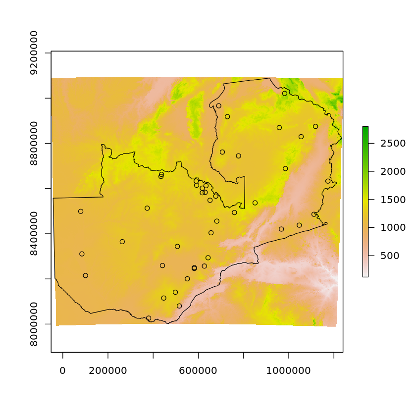
We’ll visualise these as well

plot(altitude)
plot(df_zambia['geometry'], add=TRUE)
plot(df_zambian_cities_UTM35S['geometry'], add=TRUE)

Voronoi Tesselation/Thiessen Polygons

Before we move on to interpolation we’ll look at how we can create a Voronoi diagram:

… a partitioning of a plane into regions based on distance to points in a specific subset of the plane. That set of points (called seeds, sites, or generators) is specified beforehand, and for each seed there is a corresponding region consisting of all points closer to that seed than to any other. - Wikipedia

We’ll now use the deldir function to carry out Delaunay triangulation and Dirichlet tessellation, this function returns a complex object.

cities_deldir <- deldir(df_zambian_cities_UTM35S$LONGITUDE, df_zambian_cities_UTM35S$LATITUDE)

cities_deldir

Delaunay triangulation and Dirchlet tessellation
of 43 data points.

Enclosing rectangular window:
[22.11,34.190001] x [-18.751667,-7.931666] 

Area of rectangular window (total area of
Dirichlet tiles):
130.7056 

Area of convex hull of points (total area of
Delaunay triangles):
54.96517 

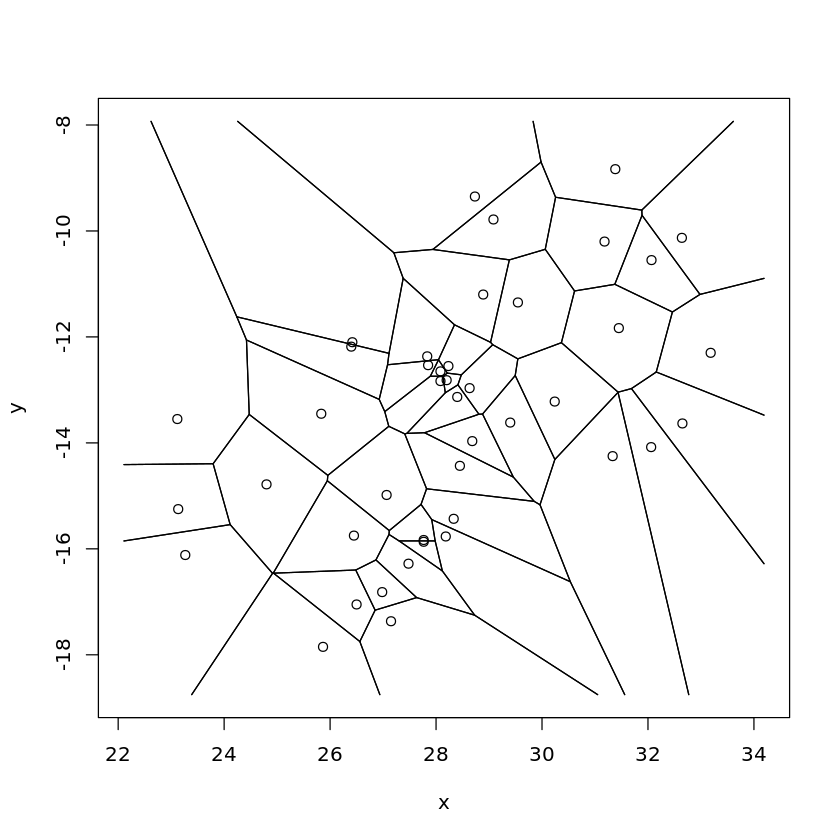
We can use tile.list to convert the complex object returned in the last step into a list where each entry is a separate Dirichlet/Voronoi tile

cities_polygons <- tile.list(cities_deldir) # Produces Thiessen polygons

plot(cities_polygons)

We can then susbset the returned object, with each element relating to a single city in the original dataset, the area attribute is the size of the Polygon for that city.

cities_polygons[[1]]

$ptNum

1

$pt

x

28.083334

y

-12.65

$x

1. 28.046429
2. 27.891667
3. 28.129763
4. 28.213637

$y

1. -12.432142
2. -12.741666
3. -12.741666
4. -12.682955

$bp

1. FALSE
2. FALSE
3. FALSE
4. FALSE

$area

0.052275

Interpolation

Before we start interpolating we’ll quickly inspect the dataset for any clear trends, starting with the lon/lat & altitude relationship with solar potential.

First we’ll extract the solar and altitude values for the points we’ve selected (just so happens to be cities in this case).

city_coords = st_coordinates(df_zambian_cities_UTM35S)

df_zambian_cities_UTM35S$solar <- extract(solar, city_coords)
df_zambian_cities_UTM35S$altitude <- extract(altitude, city_coords)

df_zambian_cities_UTM35S$x <- city_coords[, 1]
df_zambian_cities_UTM35S$y <- city_coords[, 2]

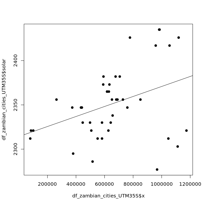
Longitude appears to have a weak relationship with solar output

plot(df_zambian_cities_UTM35S$x, df_zambian_cities_UTM35S$solar, pch=19)
abline(lm(df_zambian_cities_UTM35S$solar ~ df_zambian_cities_UTM35S$x))

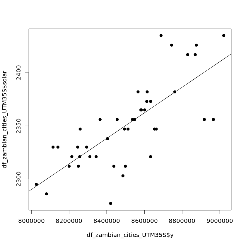
Latitude appears to have a stronger relationship with solar output which would be expected (why do you think this is?).

plot(df_zambian_cities_UTM35S$y, df_zambian_cities_UTM35S$solar, pch=19)
abline(lm(df_zambian_cities_UTM35S$solar ~ df_zambian_cities_UTM35S$y))

We’ll now create a model that predicts solar based on a 1st order linear regression against longitude/latitude.

trend_1st <- lm(solar~x+y, data=df_zambian_cities_UTM35S)
summary(trend_1st)

Call:
lm(formula = solar ~ x + y, data = df_zambian_cities_UTM35S)

Residuals:
    Min      1Q  Median      3Q     Max 
-63.083  -9.265   1.744  19.652  62.488 

Coefficients:
              Estimate Std. Error t value Pr(>|t|)    
(Intercept)  1.321e+03  1.605e+02   8.230 3.87e-10 ***
x           -1.636e-06  1.804e-05  -0.091    0.928    
y            1.212e-04  1.954e-05   6.203 2.45e-07 ***
---
Signif. codes:  0 ‘***’ 0.001 ‘**’ 0.01 ‘*’ 0.05 ‘.’ 0.1 ‘ ’ 1

Residual standard error: 26.87 on 40 degrees of freedom
Multiple R-squared:  0.5649,	Adjusted R-squared:  0.5432 
F-statistic: 25.97 on 2 and 40 DF,  p-value: 5.903e-08

We’ll now create a grid that we will carry out the predictions over

grid <- st_as_sf(rasterToPoints(solar, spatial=TRUE)) # uses existing raster cell centres as point locations
grid$solar <- NULL # clear existing data

plot(grid, pch=".")

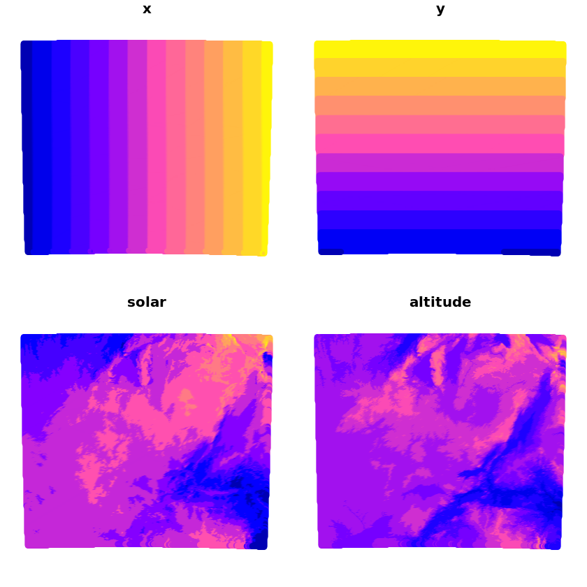
We’ll now populate this empty grid with the x/y values and solar/altitude values

grid_coords <- as.data.frame(st_coordinates(grid))

grid$x <- grid_coords[, 1]
grid$y <- grid_coords[, 2]

grid$solar <- extract(solar, grid_coords[, 1:2])
grid$altitude <- extract(altitude, grid_coords[, 1:2])

plot(grid)

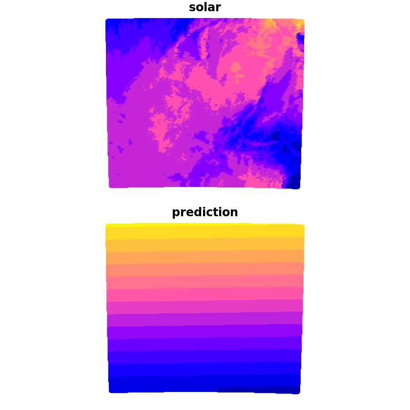
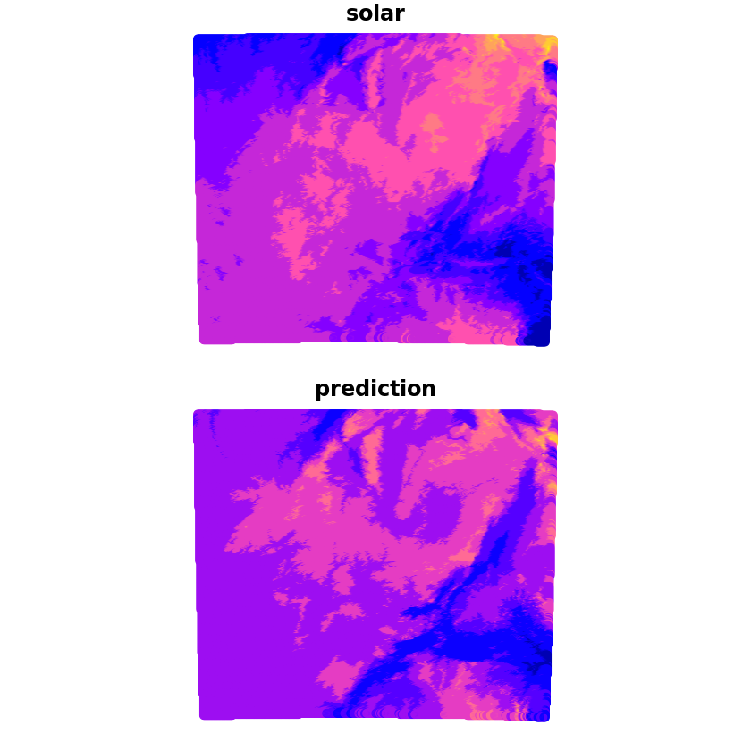
We can now make the prediction which we’ll compare with the true solar values, we can see that whilst it captures some of the wider characteristics there are a lot of discrepancies still.

grid_pred <- predict(trend_1st, newdata=grid, se.fit=TRUE)
grid$prediction <- grid_pred$fit

plot(grid[c('solar', 'prediction')])

We don’t just have to regress against longitude/latitude though, here we’ll repeat the previous steps but only use latitude as a regressor.

First we’ll visualise the relationship between the two.

plot(df_zambian_cities_UTM35S$altitude, df_zambian_cities_UTM35S$solar, pch=19)
abline(lm(df_zambian_cities_UTM35S$solar ~ df_zambian_cities_UTM35S$altitude))

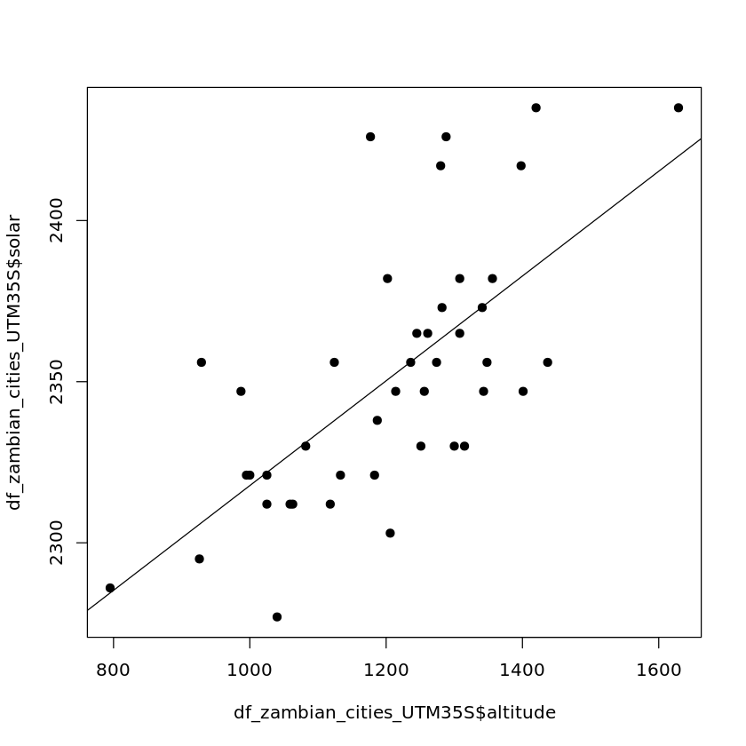
Then we’ll fit a model and use it in our prediction.

trend_1st <- lm(solar~altitude, data=df_zambian_cities_UTM35S)

grid_pred <- predict(trend_1st, newdata=grid, se.fit=TRUE)
grid$prediction <- grid_pred$fit

plot(grid[c('solar', 'prediction')])

Questions

Best Fit Model

• What combination of the inputs produces the most accurate results?

• Should we use the standard r2 score or the adjusted r2 score?

• How do the results change when you use a test/train split?

• How could we improve over a random sample on the test/train split? (Think about what you would do with time-series cross-validation)

# 

previous

Working with Raster Data

next

Coursework Support